Support Vector Machines (SVMs) are fundamentally linear classifiers designed to find the optimal hyperplane that separates data points belonging to different classes. This hyperplane is not just any boundary; it is chosen to maximize the margin, or the distance between the closest points from each class, which are aslso called support vectors. They are separators because they always create a linear decision boundary, or hyperplane, within the space they operate.
How kernels work
First, let me define what a kernel is. A kernel is a function that computes the dot products of data points in a transformed feature space, enabling Support Vector Machines (SVMs) to classify data that is not linearly separable in its original space.
Why dot product is critical to the use of kernel
it is important tbecause it allows us to measure similarity between data points in higher-dimensional spaces without actually computing those dimensions. All calculations can be expressed solely in terms of dot products between data points, which means we can replace every dot product with a kernel function that implicitly computes similarity in a transformed space. in short, dot products enable kernels to transform linear SVMs into non-linear classifiers without the computational cost of higher dimensions.
Polynomial Kernel Transformation: Mapping 2D Points to Higher Dimensions
r=1 and d=2
the bias=r=1
degree= d=2
For transforming a single point (x₁,x₂), this kernel formula tells us what features we need in our higher dimensional space. When d=2, we get these features:
- x₁² (square of first coordinate)
- x₂² (square of second coordinate)
- √2x₁x₂ (cross term)
Let’s take a point (3,2):
Starting with (x₁, x₂) = (3,2), we apply the transformation based on d=2:
- x₁² = 3² = 9
- x₂² = 2² = 4
- √2x₁x₂ = √2 × 3 × 2 = √2 × 6 ≈ 8.49
So the 2D point (3,2) transforms into the 3D point (9, 4, 8.49)

Figure 1: illustrates the transformation of the 2D point (3,2) into 3D space (9,4,8.49) using a polynomial kernel with parameters r=1 and d=2. The kernel maps the original point into a higher-dimensional space using the transformation (x₁²,x₂²,√2x₁x₂).
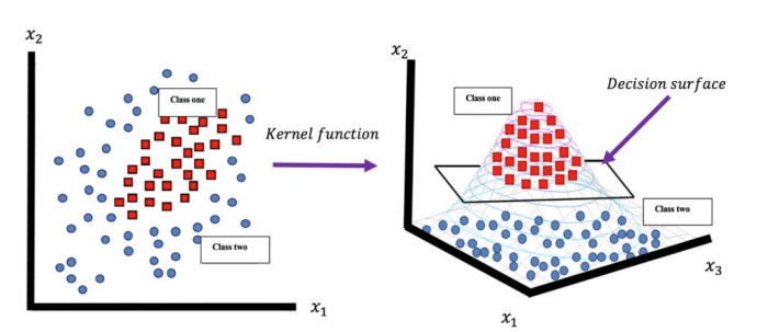
Figure 2: illustrates how a kernel function transforms non-linearly separable 2D data into linearly separable data in higher dimensional space, where a decision surface can separate the two classes.
source:https://doi.org/10.21123/bsj.2020.17.4.1255
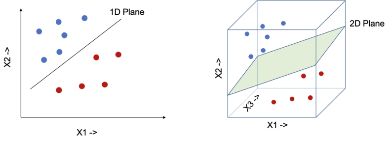
Figure 3: visualizes a hyperplane separating blue and red data points in multiple dimensions
Data Prep
Before
Link to the data before cleaning: Exclusive_Location_ProteinsV1.xlsx
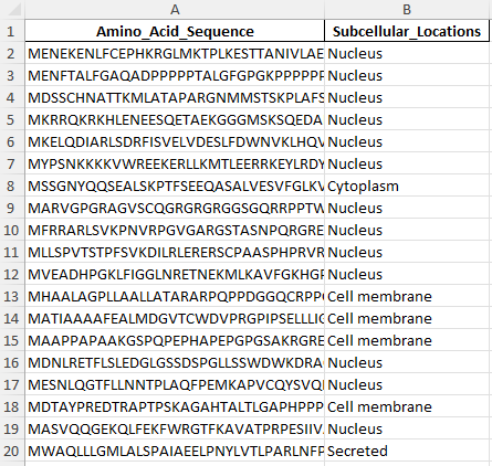
The dataset consists of two columns: Amino_Acid_Sequence and Subcellular_Locations. The Amino_Acid_Sequence column contains the primary sequences of proteins, while the Subcellular_Locations column specifies the subcellular compartment where each protein is localized (e.g., Nucleus, Cytoplasm, Cell membrane, or Secreted). This raw data will require transformation into a numerical format suitable for SVM modeling.
After
Link to the data after cleaning: processed_V1.xlsx
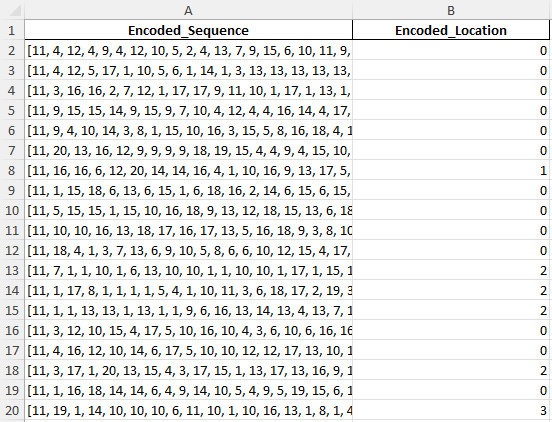
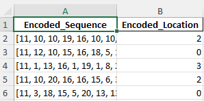
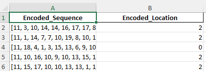
Here I transformed the dataset for SVM modeling by encoding Amino_Acid_Sequence into numeric representations of amino acids and mapping Subcellular_Locations to unique integers. The processed data now contains two columns: Encoded_Sequence and Encoded_Location, ready for supervised learning.
The dataset was divided into a training set (80%) and a testing set (20%) to ensure that the model is evaluated on unseen data, thereby providing an unbiased measure of its performance. This disjoint split is critical in supervised learning to avoid data leakage and ensure the model generalizes well to new data. Additionally, SVM requires numeric data for both features and labels. To meet this requirement, Amino_Acid_Sequence was encoded into numeric vectors, and Subcellular_Locations was mapped to unique integers. This ensures the data is compatible with SVM and ready for supervised learning.
Example train data
Example test data
Code
This is the code that generated the ouput above.
Link to the input excel file: Exclusive_Location_ProteinsV1.xlsx
Link the ouput excel file:processed_V1.xlsx
import pandas as pd
from sklearn.model_selection import train_test_split
from sklearn.svm import SVC
from sklearn.metrics import classification_report, confusion_matrix, accuracy_score
import matplotlib.pyplot as plt
import seaborn as sns

file_path = "path_to_processed_V1.xlsx"
df = pd.read_excel(file_path)


X = df['Encoded_Sequence'].apply(lambda x: eval(x)).tolist()
y = df['Encoded_Location']

X_train, X_test, y_train, y_test = train_test_split(X, y, test_size=0.2, random_state=42)

from sklearn.preprocessing import MultiLabelBinarizer
mlb = MultiLabelBinarizer()
X_train = mlb.fit_transform(X_train)
X_test = mlb.transform(X_test)

kernels = ['linear', 'poly', 'rbf']
results = {}


for kernel in kernels:
    svm = SVC(kernel=kernel, random_state=42)
    svm.fit(X_train, y_train)
    y_pred = svm.predict(X_test)


    acc = accuracy_score(y_test, y_pred)
    cm = confusion_matrix(y_test, y_pred)
    report = classification_report(y_test, y_pred, output_dict=True)


    results[kernel] = {
        'accuracy': acc,
        'confusion_matrix': cm,
        'classification_report': report
    }


    print(f"Kernel: {kernel}")
    print(f"Accuracy: {acc}")
    print("Classification Report:")
    print(pd.DataFrame(report).transpose())
    print("\n")


for kernel in kernels:
    plt.figure(figsize=(6, 6))
    sns.heatmap(results[kernel]['confusion_matrix'], annot=True, fmt='d', cmap='YlOrBr', cbar=True)
    plt.title(f"Confusion Matrix_{kernel.capitalize()} Kernel", fontsize=14)
    plt.xlabel("Predicted", fontsize=12)
    plt.ylabel("Actual", fontsize=12)
    plt.savefig(f"path_to_save/Confusion_Matrix_{kernel.capitalize()}_Kernel.png")
    plt.show()

kernel_names = list(results.keys())
accuracies = [results[kernel]['accuracy'] for kernel in kernels]

plt.figure(figsize=(8, 5))
plt.bar(kernel_names, accuracies, color='gold')
plt.title("Accuracy Comparison Across Kernels", fontsize=14)
plt.xlabel("Kernel", fontsize=12)
plt.ylabel("Accuracy", fontsize=12)
plt.savefig("path_to_save/Comparing_accuracy.png")
plt.show()
Results


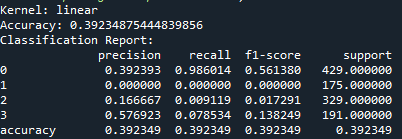

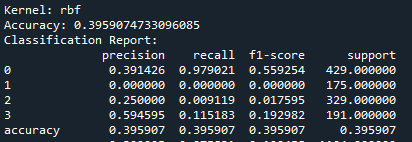
What does this mean?
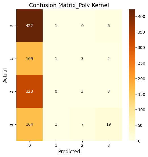
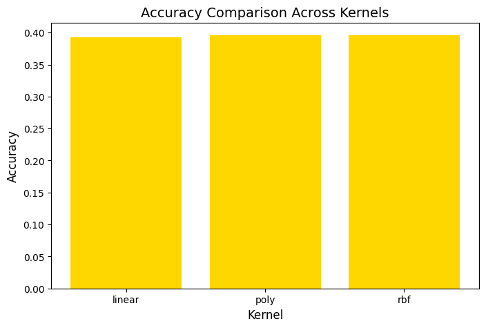
So, basically, the SVM was run using three kernels: linear, polynomial, and RBF and all three kernels performed similarly in terms of accuracy. The polynomial and RBF kernels achieved an accuracy of 39.6%, while the linear kernel reached 39.2%. The model showed the highest recall for class 0, which represents proteins localized in the nucleus. However, it struggled with other locations, including the cytoplasm (class 1), cell membrane (class 2), and secreted proteins (class 3). The weighted F1-scores ranged between 0.242 and 0.251. This highlights challenges in predicting proteins in less dominant locations. Improving the feature set or addressing class imbalances could enhance the model’s performance.
Note: I did do a Sigmoid as a fourth kernel.
kernels = [‘linear’, ‘poly’, ‘rbf’, ‘sigmoid’] that resulted in 38.17%.
Conclusions
IT seems like the SVM algorithm used may not be complex enough to capture the intricate biological patterns in subcellular localization data. While there is sufficient data for all four classes, class imbalance causes overrepresentation of the nucleus and underrepresentation of other locations, leading to skewed predictions. Furthermore, the encoded sequence features might lack the depth needed to differentiate subtle biological differences between locations. It might be wise exploring more advanced algorithms, such as neural networks. It might better handle the complexity of the data.
