Multinomial Naïve Bayes is a classification algorithm that predicts categories based on probabilities from past data, assuming each feature is independent of the others. The “naïve” in the name is there because it simplifies by treating features as unrelated, even though they often are. This assumption allows the model to perform quick probability calculations, making it effective and efficient for large datasets. For instance, one decent example is a doctor trying to figure out if a patient has a particular disease based on their symptoms like fever, cough, and fatigue. A Naïve Bayes model would look at each symptom separately, as if they were completely unrelated. It would calculate the chance of the disease based on how often each symptom has shown up in people with the disease in the past. So, if fever, cough, and fatigue are common in people with the flu, the model would think it’s very likely that the patient has the flu if they have all three symptoms. However, the model wouldn’t consider that these symptoms often go together. It would treat them as if they were independent(most likely not representative of real life).

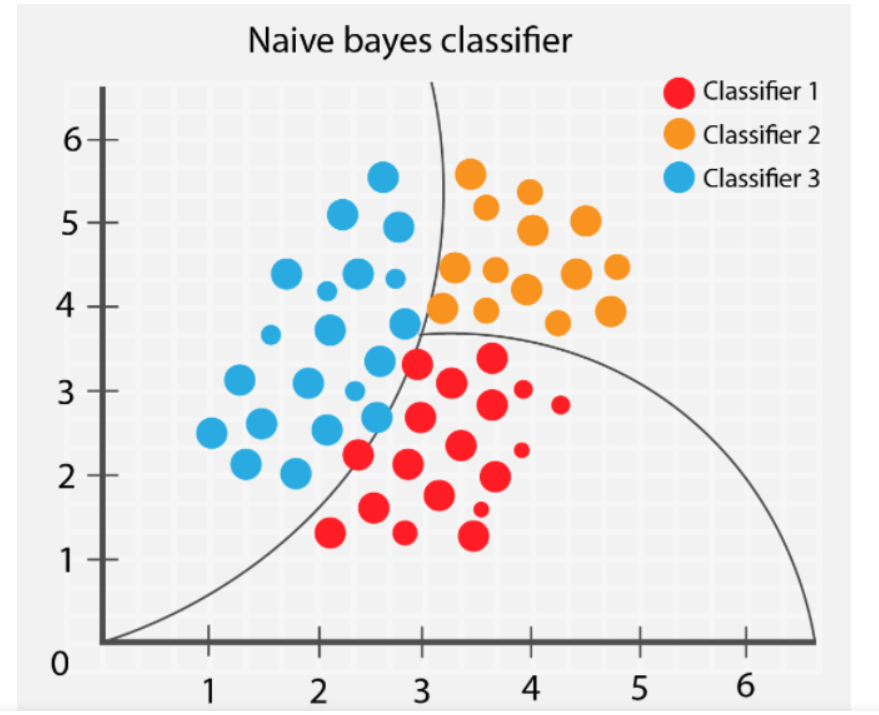
Figure 1: The image illustrates a Naïve Bayes classifier dividing data points into three classes: Classifier 1 (red), Classifier 2 (orange), and Classifier 3 (blue). The curved decision boundaries separate the classes based on probability distributions. The classifier assigns each point to the most probable class, given its position, by assuming that features are independent.
Source: https://www.linkedin.com/pulse/naive-bayes-classifier-beginners-guide-muqadas-rasheed-/
Bernoulli Naïve Bayes: type of Naïve Bayes mainly meant for binary data. The algorithm assumes that all features are independent of each other just like the above and uses the Bernoulli distribution to model the probability of each feature’s presence or absence for each class.

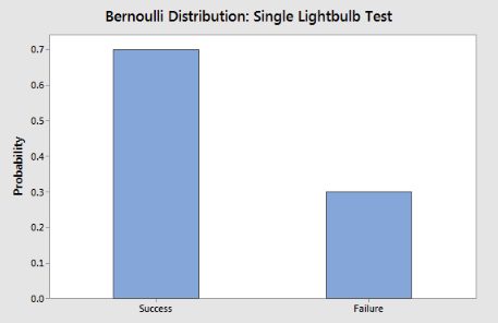
Figure 2:The figure above displays a Bernoulli distribution for a “Single Lightbulb Test,” showing the probabilities of “Success” (lightbulb works) and “Failure” (lightbulb doesn’t work). This type of distribution is fundamental to Bernoulli Naïve Bayes, which uses binary outcomes to model the likelihood of feature presence or absence for each class.
source: https://statisticsbyjim.com/probability/bernoulli-distribution/
Smoothing: it is a technique used to avoid zero probabilities for features that don’t appear in the training data. This prevents the model from making incorrect predictions when it encounters unseen data. Laplace smoothing adds a small constant(most of the time 1) to feature counts, ensuring that no probability is zero. This allows the model to make more reliable predictions, even with limited data.
NB data prep
Proteins can localize to multiple compartments within a cell; to simplify prediction and make the data cleaner, the dataset was filtered to include only proteins known to localize to a single compartment. This approach ensures that proteins used downstream have one known localization based on available information. The focus was placed on four localizations with the largest sample sizes and relevance: Nucleus, Cytoplasm, Cell membrane, and Secreted.
Python code to clean the data
import pandas as pd

# Loading the original Excel file
file_path = r"path_to_Cleaned_raw_2.xlsx"
data = pd.read_excel(file_path)

# Defining the localizations we want to keep
exclusive_locations = ["Nucleus", "Cytoplasm", "Cell membrane", "Secreted"]

# Filtering for proteins localized exclusively in one of the specified locations
filtered_data = data[
    data['Subcellular_Locations']
    .str.replace(',', ';')
    .str.split(';')
    .apply(lambda locations: len(locations) == 1 and locations[0].strip() in exclusive_locations)
][['Amino_Acid_Sequence', 'Subcellular_Locations']]

# Saving the filtered data to a new Excel file
output_file_path = r"D:\module_3_proj\Exclusive_Location_Proteins_Updated.xlsx"
filtered_data.to_excel(output_file_path, index=False)
print(f"Filtered data saved to {output_file_path}")

# Printing counts of each localization in the terminal
localization_counts = filtered_data['Subcellular_Locations'].value_counts()
print("Localization Counts:\n", localization_counts)
Before:
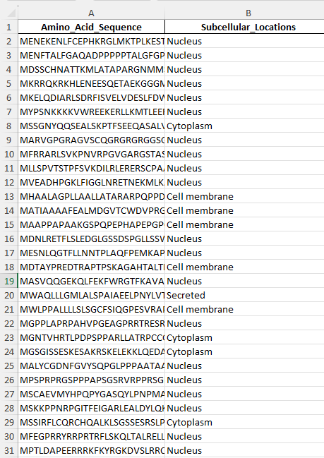
Many columns not relevant for the prediction(except Amino_Acid_Sequence and Subcellular_Locations) exist that need to be removed.
link to the original: Cleaned_raw_2.xlsx

After:
This is what remains after the removal.

Link: Exclusive_Location_ProteinsV1.xlsx
Data Preparation and Stratified Split for Protein Subcellular Localization Prediction
The data was split using a stratified 80-20 split to ensure balanced representation of each localization class in both the training and testing sets. This, of course, ensures that each localization type is proportionally represented in both training and testing sets. allowing the model to learn from a balanced dataset and be accurately evaluated across all categories.
Creating a disjoint split, with no overlap between training and testing sets, ensures the model is evaluated on entirely new protein sequence data. This approach prevents information from the training sequences from influencing test results.
Python code
import pandas as pd
from sklearn.model_selection import train_test_split
from sklearn.preprocessing import LabelEncoder

# Loading the filtered data with the updated file name
file_path = r"path_to_Exclusive_Location_ProteinsV1.xlsx"
filtered_data = pd.read_excel(file_path)

# Encoding the Subcellular_Locations into numerical labels
label_encoder = LabelEncoder()
filtered_data['Location_Code'] = label_encoder.fit_transform(filtered_data['Subcellular_Locations'])

# Splitting data into training and testing sets with stratification
X = filtered_data['Amino_Acid_Sequence']
y = filtered_data['Location_Code']

# Perform a stratified split to ensure each localization is represented 80/20
X_train, X_test, y_train, y_test = train_test_split(X, y, test_size=0.2, random_state=42, stratify=y)

# Displaying label mappings and the new split counts for reference
label_mappings = dict(zip(label_encoder.classes_, label_encoder.transform(label_encoder.classes_)))
print("Label mappings:", label_mappings)
print(f"Training set size: {len(X_train)}, Testing set size: {len(X_test)}")

# Displaying counts of each localization in the training and testing sets
print("Training set distribution:\n", y_train.value_counts())
print("Testing set distribution:\n", y_test.value_counts())
Output of the 80/20 split.
Training Set Distribution:
- Nucleus: 1769
- Cell membrane: 1273
- Secreted: 769
- Cytoplasm: 684
Testing Set Distribution:
- Nucleus: 442
- Cell membrane: 319
- Secreted: 192
- Cytoplasm: 171
Protein Localization Prediction using k-mer Encoding and Multinomial Naïve Bayes
import pandas as pd
from sklearn.model_selection import train_test_split
from sklearn.preprocessing import LabelEncoder
from sklearn.feature_extraction.text import CountVectorizer
from sklearn.naive_bayes import MultinomialNB
from sklearn.metrics import accuracy_score, confusion_matrix

# Loading the filtered data
file_path = r"path_to_Exclusive_Location_ProteinsV1.xlsx"
data = pd.read_excel(file_path)

# Encoding subcellular locations as numerical labels
label_encoder = LabelEncoder()
data['Location_Code'] = label_encoder.fit_transform(data['Subcellular_Locations'])

# Splitting data into training and testing sets with stratification
X = data['Amino_Acid_Sequence']  # Input sequences
y = data['Location_Code']        # Encoded labels
X_train, X_test, y_train, y_test = train_test_split(X, y, test_size=0.2, random_state=42, stratify=y)

# Defining a function to generate k-mers from sequences (using 3-mers here)
def get_kmers(sequence, k=3):
    return [sequence[i:i+k] for i in range(len(sequence) - k + 1)]

# Converting sequences into 3-mers for training and testing
X_train_kmers = [' '.join(get_kmers(seq, k=3)) for seq in X_train]
X_test_kmers = [' '.join(get_kmers(seq, k=3)) for seq in X_test]

# Using CountVectorizer to create k-mer count features
vectorizer = CountVectorizer()
X_train_features = vectorizer.fit_transform(X_train_kmers)
X_test_features = vectorizer.transform(X_test_kmers)

# Training the Multinomial Naïve Bayes model
model = MultinomialNB()
model.fit(X_train_features, y_train)

# Making predictions on the test set
y_pred = model.predict(X_test_features)

# Evaluating the model
accuracy = accuracy_score(y_test, y_pred)
conf_matrix = confusion_matrix(y_test, y_pred)

# Printing results
print(f"Accuracy: {accuracy:.2f}")
print("Confusion Matrix:")
print(conf_matrix)

# Showing label mappings for reference
label_mappings = dict(zip(label_encoder.classes_, label_encoder.transform(label_encoder.classes_)))
print("Label mappings:", label_mappings)
Output

Summary
The model achieved an accuracy of 68% in predicting protein locations within a cell. It performed well in identifying nuclear proteins but sometimes confused them with proteins localized to the cytoplasm or cell membrane. Considering the complexity of this task, the model’s performance is reasonable, though there is room for improvement. Increasing accuracy may involve using larger k-mers or more advanced encoding techniques to capture additional sequence context. However, protein sequences are inherently complex, and certain localization signals may be subtle or not fully evident from the sequence alone, which presents a technical limitation.
