This ML technique is where many models are combined together in an ‘ensemble’ to improve overall performance.Though the aggregation of predictions from multiple models, robustness is increased. Some of the methods used are bagging, boosting, stacking, and voting. Boosting trains models sequentially, where each subsequent model corrects the errors of the previous one, while bagging trains models in parallel using random subsets of the data. .
Example
Boosting is as technique where models are trained sequentially where the error of the prior model is corrected by the next model that will take in the weighted data points with higher weight assigned to misclassification. The goal is that by the end of the training process the ensemble of models would have leant to accurately predictive model.
Bagging uses a different method where models are trained in parallel(not sequential) using random subsets of the training data through bootstrap sampling. In this ensemble each model is trained separately, and their predictions are combined through voting/averaging to create to bus model that reduces variance. In short, the predictions are aggregated from all individual models hence bootstrap aggregating or bagging.
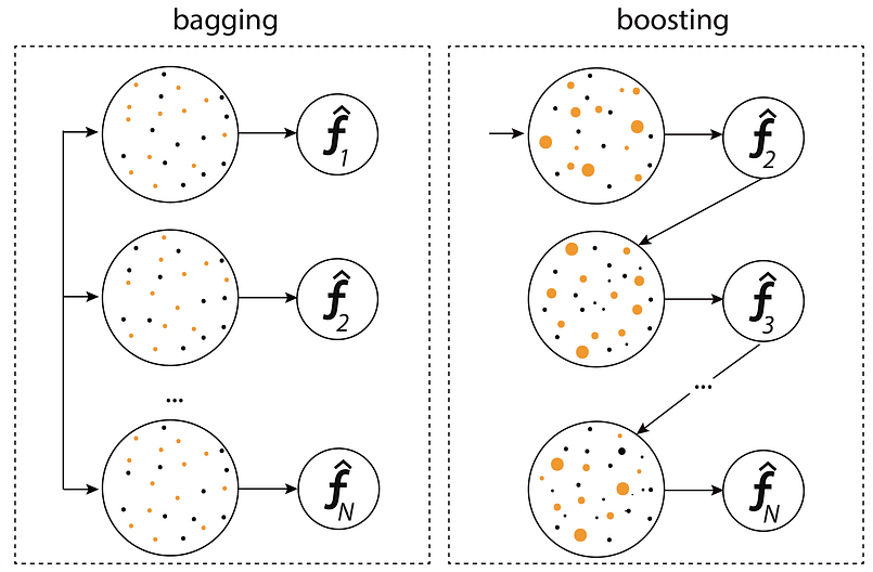
Here the figure shows the parallel training process in bagging, where models are trained independently on random subsets of data, compared to the sequential process in boosting, where each model corrects the errors of its predecessor.
Code
1st Model
XGboost
The python code below applies XGBoost.
import pandas as pd
from sklearn.model_selection import train_test_split
from sklearn.metrics import classification_report, confusion_matrix, accuracy_score
import matplotlib.pyplot as plt
import seaborn as sns
from xgboost import XGBClassifier

file_path = "C:/Users/GAMING PC/Downloads/for_SVM/processed_V1.xlsx"
df = pd.read_excel(file_path)


X = df['Encoded_Sequence'].apply(lambda x: eval(x)).tolist()
y = df['Encoded_Location']


from sklearn.preprocessing import MultiLabelBinarizer
mlb = MultiLabelBinarizer()
X = mlb.fit_transform(X)

X_train, X_test, y_train, y_test = train_test_split(X, y, test_size=0.2, random_state=42)

xgb = XGBClassifier(eval_metric='mlogloss', random_state=42)
xgb.fit(X_train, y_train)

y_pred = xgb.predict(X_test)

accuracy = accuracy_score(y_test, y_pred)
print(f"Accuracy: {accuracy}")
print("\nClassification Report:")
print(classification_report(y_test, y_pred))

cm = confusion_matrix(y_test, y_pred)
plt.figure(figsize=(6, 6))
sns.heatmap(cm, annot=True, fmt='d', cmap='pink', cbar=True)
plt.title("Confusion Matrix - XGBoost", fontsize=14)
plt.xlabel("Predicted", fontsize=12)
plt.ylabel("Actual", fontsize=12)
plt.show()

feature_importance = xgb.feature_importances_
plt.figure(figsize=(10, 6))
plt.bar(range(len(feature_importance)), feature_importance, color='pink')
plt.title("Feature Importance - XGBoost", fontsize=14)
plt.xlabel("Feature Index", fontsize=12)
plt.ylabel("Importance", fontsize=12)
plt.show()
Results for XGBoost
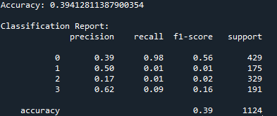
Note: I explored two modifications to address the class imbalance issue. First, I applied SMOTE-based oversampling, which generates synthetic samples for the minority classes to balance the training data. Second, I implemented cost-sensitive learning by adjusting class weights to penalize misclassifications of underrepresented classes. Both approaches aimed to improve the model’s ability to classify minority classes, such as Cytoplasm, Cell Membrane, and Secreted proteins. However, neither modification resulted in a significant improvement, with the accuracy remaining approximately 39.5%. This suggests that the feature representation or inherent separability of the data may be the primary limitations, rather than the class imbalance alone.
2nd model
Bagging
import pandas as pd
import numpy as np
from sklearn.model_selection import train_test_split
from sklearn.metrics import classification_report, confusion_matrix, accuracy_score
import matplotlib.pyplot as plt
import seaborn as sns
from sklearn.ensemble import BaggingClassifier
from sklearn.tree import DecisionTreeClassifier

file_path = "C:/Users/GAMING PC/Downloads/for_SVM/processed_V1.xlsx"
df = pd.read_excel(file_path)


X = df['Encoded_Sequence'].apply(lambda x: eval(x)).tolist()
y = df['Encoded_Location']

from sklearn.preprocessing import MultiLabelBinarizer
mlb = MultiLabelBinarizer()
X = mlb.fit_transform(X)

X_train, X_test, y_train, y_test = train_test_split(X, y, test_size=0.2, random_state=42)

bagging = BaggingClassifier(
    estimator=DecisionTreeClassifier(),
    n_estimators=100,
    max_samples=0.8,
    max_features=0.8,
    random_state=42
)
bagging.fit(X_train, y_train)


y_pred = bagging.predict(X_test)

accuracy = accuracy_score(y_test, y_pred)
print(f"Accuracy: {accuracy}")
print("\nClassification Report:")
print(classification_report(y_test, y_pred))

plt.figure(figsize=(6, 6))
sns.heatmap(confusion_matrix(y_test, y_pred),
            annot=True,
            fmt='d',
            cmap='Greens',
            cbar=True)
plt.title("Confusion Matrix - Bagging Classifier", fontsize=14)
plt.xlabel("Predicted", fontsize=12)
plt.ylabel("Actual", fontsize=12)
plt.show()

feature_importance = np.mean([tree.feature_importances_
                            for tree in bagging.estimators_
                            if hasattr(tree, 'feature_importances_')],
                           axis=0)

plt.figure(figsize=(10, 6))
plt.bar(range(len(feature_importance)), feature_importance, color='green')
plt.title("Average Feature Importance - Bagging Classifier", fontsize=14)
plt.xlabel("Feature Index", fontsize=12)
plt.ylabel("Importance", fontsize=12)
plt.show()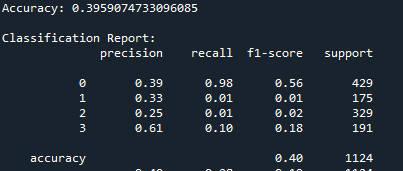
The Accuracy result from the XGBoost and Bagging classifier is around 39.6%. There is not much difference.
Results
XGBoost confusion matrix
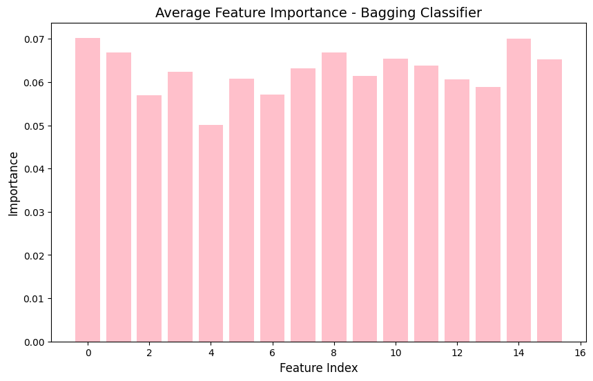
XGBoost feature importance graph
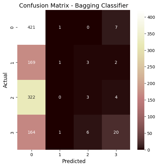
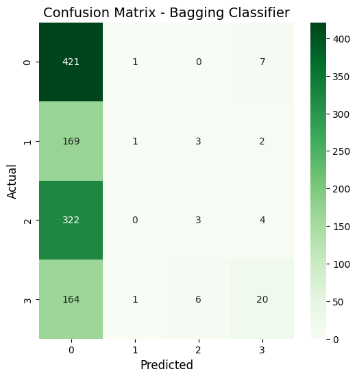
Bagging classifier confusion matrix
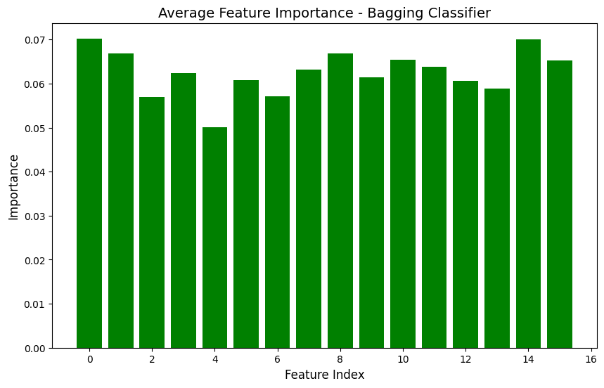
Bagging classifiers feature importance graph
Summary
in short, through the analysis of the XGBoost and Bagging classifiers,it is apparent that they both got similar accuracies of around 39.6%. When I look at the confusion matrices, I can see that both models are mostly predicting class 0, which means I probably have a class imbalance issue to deal with. Looking at the feature importance plots, I noticed that all my features have pretty similar importance values between 0.05 and 0.07, so none of them are standing out as super important for predictions. Based on these results, I think my location prediction task is pretty tricky, probably because the features for different locations are too similar. To improve this, I might need to work on the class imbalance problem and maybe come up with better features.
***Biology is a little complex for some of these models tested***
