It is a supervised learning algorithm that resembles an inverted tree(figure 1), breaking down decisions into branches based on features in a data. It starts with a root node and branches out into internal nodes, each representing a decision point. These internal nodes split the data based on specific conditions, leading to leaf nodes that represent the final decision or classification.
Example
In a Decision Tree classifying whether a protein localizes to the nucleus or cytoplasm, the root node might consider the presence of a particular amino acid pattern. If this pattern is present, the tree branches one way, leading to further nodes with questions about additional sequence features. Eventually, the branching path leads to a leaf node, which makes the final prediction(such as “nucleus” or “cytoplasm”) based on the observed features. This mimics human-like decision-making by following a set of logical steps to reach a conclusion.
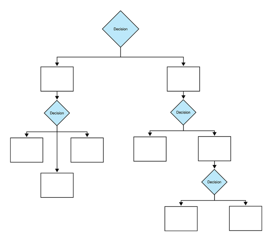
Figure 1: The diagram shows a hierarchical tree structure with decision nodes branching into multiple paths.
Discussing how and why gini, entropy and Information gain are used.
To construct a decision tree, the algorithm needs to determine the best way to split the data at each node. This is where Gini impurity, entropy, and information gain come into play. These metrics help assess the quality of a potential split.
#1 Gini Impurity is a measure used in Decision Trees to evaluate how “pure” a node is. “Purity” here means how much of a single class (or label) is present in a node. If a node is perfectly pure, all data points within it belong to the same class, and the Gini impurity is 0. If the classes are mixed, the Gini impurity increases.
#2 Entropy :Entropy refers to the randomness or uncertainty in a dataset. The higher the entropy, the more uncertainty in the data, and vice versa.
#3 Information gain: This is a way to calculate the reduction in entropy achieved by a split. Higher information gain is good as it is more able to separate the data into distinct classes. It is calculated as the difference between the entropy before and after a split.
So, to build effective decision trees, algorithms rely on metrics like Gini impurity, entropy, and information gain. Gini impurity measures the impurity of a node, while entropy measures the randomness or uncertainty. Information gain quantifies the reduction in uncertainty achieved by a split. By optimizing these metrics, decision trees can create accurate and interpretable models.
For protein localization data, Gini impurity or entropy helps the Decision Tree find the best splits to separate localization types, like Nucleus and Cytoplasm. For example, if a specific 3-mer pattern strongly indicates nuclear proteins, the tree can split on this feature to create purer groups for each class. By maximizing information gain, the tree builds more accurate branches to predict where proteins are located.
DT data prep and code
Cleaned data
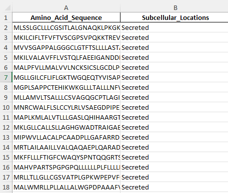
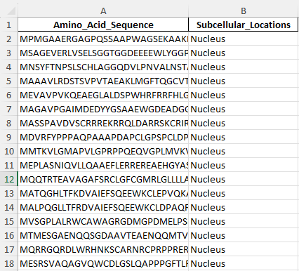
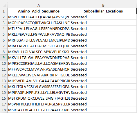
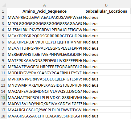
Image of the sample train and test data to be used.
Training data
Example train data for the proteins secreted outside of a cell. This is 1/4 locations I am predicting for.
Example train data for the proteins in the nucleus. This is 1 of 4 locations I am predicting for.
Test data
Example rest data for the proteins secreted outside of a cell.
Example test data for the proteins in the nucleus.
Python code to run the DT algorithm
link to excel file used as an input: Exclusive_Location_ProteinsV1.xlsx
import pandas as pd
from sklearn.model_selection import train_test_split
from sklearn.preprocessing import LabelEncoder
from sklearn.feature_extraction.text import CountVectorizer
from sklearn.tree import DecisionTreeClassifier
from sklearn.metrics import accuracy_score, confusion_matrix

# Loading the filtered data
file_path = r"path_to_Exclusive_Location_ProteinsV1.xlsx"
data = pd.read_excel(file_path)

# Converting location labels to numerical codes
label_encoder = LabelEncoder()
data['Location_Code'] = label_encoder.fit_transform(data['Subcellular_Locations'])

# Splitting into 80% training and 20% testing, keeping class proportions equal
X = data['Amino_Acid_Sequence']
y = data['Location_Code']
X_train, X_test, y_train, y_test = train_test_split(X, y, test_size=0.2, random_state=42, stratify=y)

# Function to create k-mers from sequences (3-mers in this case)
def get_kmers(sequence, k=3):
    return [sequence[i:i+k] for i in range(len(sequence) - k + 1)]

# Converting sequences into 3-mers for train and test data
X_train_kmers = [' '.join(get_kmers(seq, k=3)) for seq in X_train]
X_test_kmers = [' '.join(get_kmers(seq, k=3)) for seq in X_test]

# Transforming 3-mers into numerical features with CountVectorizer
vectorizer = CountVectorizer()
X_train_features = vectorizer.fit_transform(X_train_kmers)
X_test_features = vectorizer.transform(X_test_kmers)

# Training the Decision Tree model
tree_model = DecisionTreeClassifier(random_state=42)
tree_model.fit(X_train_features, y_train)

# Making predictions on the test set
y_tree_pred = tree_model.predict(X_test_features)

# Evaluating the model
tree_accuracy = accuracy_score(y_test, y_tree_pred)
tree_conf_matrix = confusion_matrix(y_test, y_tree_pred)

# Printing accuracy and confusion matrix
print(f"Decision Tree Accuracy: {tree_accuracy:.2f}")
print("Decision Tree Confusion Matrix:")
print(tree_conf_matrix)
summary
The train-test split used an 80-20 ratio with stratification to keep class proportions balanced in both sets, ensuring each localization type was well represented. This disjoint split, with no overlap between training and testing data, prevents data leakage and allows for an accurate evaluation on unseen data.
DT results and conclusions
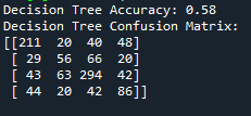
From the results above, we can see that the Decision Tree model achieved an accuracy of 58%, which indicates a moderate level of success in predicting protein localization. The confusion matrix shows that the model was particularly accurate in identifying Nucleus proteins, with 294 correct classifications, but had more difficulty with Cytoplasm and Secreted proteins, which were often misclassified. The misclassification might point to existence of some overlap in sequence patterns, making it challenging for the model to differentiate these categories. In a nut shell, the results highlight that while the model captures some localization signals, there is room for improvement, possibly by incorporating additional features or using more complex models.
