Fetch Reviewed Human Protein Data from UniProt with Python
import requests
import pandas as pd
import io
import gzip

### Setting up the API request
#This endpoint is used to stream data from UniProt withe the parameters that are sepcified
url = "https://rest.uniprot.org/uniprotkb/stream"
params = {
    "format": "tsv",
    "fields": "accession",
  # For reviewed proteins from Homo sapiens
    "query": "(organism_id:9606) AND (reviewed:true)",
    "compressed": "true"
}

### Making the request
response = requests.get(url, params=params)

### Checking if the request was successful
if response.status_code == 200:
    decompressed_content = gzip.decompress(response.content)

    ### Creating a StringIO object from the decompressed content
    tsv_file = io.StringIO(decompressed_content.decode('utf-8'))

    ### Reading the TSV data into a pandas DataFrame
    df = pd.read_csv(tsv_file, sep='\t')

    ### Saving the DataFrame to a CSV file
    df.to_csv('Human_protein_id.csv', index=False)
else:
    print(f"Error: {response.status_code}")
    print(response.text)
This Python code imports the requests, pandas, io, and gzip libraries to fetch and process data from the UniProt API. It sets up a request to retrieve reviewed human protein data in compressed TSV format. After making the request, it decompresses the gzipped content if the request is successful. The decompressed data is then read into a pandas DataFrame and saved to a CSV file named human_protein_ids.csv. This code efficiently handles data retrieval and storage for reviewed human proteins.
Link to the csv file with all the human uniprot protein IDs : Human_protein_id.csv
There are 20,453 unique proteins as you can see in the csv file.
Comprehensive Protein Information Retriever from UniProt
This is going be a long code that is designed to handle several task but structured logically.
import requests
import pandas as pd
from Bio.SeqUtils.ProtParam import ProteinAnalysis
from collections import Counter
import time  # For rate limiting
import os
import re  # For regular expressions

# Fetches amino acid sequences from UniProt in FASTA format using the requests library.
# If a sequence cannot be retrieved due to an invalid ID or server issue),
# the function returns None, allowing the script to continue without crashing.
def get_uniprot_sequence(uniprot_id):
    base_url = "https://rest.uniprot.org/uniprotkb/"
    url = f"{base_url}{uniprot_id}.fasta"

    response = requests.get(url)

    if response.status_code == 200:
        fasta_content = response.text
        lines = fasta_content.strip().split('\n')
        sequence = ''.join(lines[1:])
        return sequence.strip()
    else:
        return None

# Fetches JSON data from UniProt to obtain detailed annotations such as protein names,
# gene names, subcellular locations, and other metadata.
# If the JSON data cannot be retrieved due to an invalid ID or server issue,
# the function returns None, allowing the script to handle the error.

def get_protein_domains(json_data):
    domain_databases = ['InterPro', 'Pfam', 'SMART', 'SUPFAM', 'Gene3D']
    protein_domains = []

    cross_references = json_data.get('uniProtKBCrossReferences', [])
    for ref in cross_references:
        if ref.get('database') in domain_databases:
            db = ref.get('database')
            domain_id = ref.get('id')
            properties = ref.get('properties', [])
            entry_name = ''
            for prop in properties:
                if prop.get('key') == 'EntryName':
                    entry_name = prop.get('value')
            if entry_name:
                protein_domains.append(f"{db}:{domain_id} ({entry_name})")
            else:
                protein_domains.append(f"{db}:{domain_id}")
    return '; '.join(protein_domains) if protein_domains else ''

# Extracts specific protein details from the fetched JSON data, including protein names,
# gene names, reviewed status, and subcellular locations.
# Helper functions are used to extract GO annotations and protein domains (example: InterPro, Pfam).

def get_go_annotations(json_data):
    go_annotations = []
    cross_references = json_data.get('uniProtKBCrossReferences', [])
    for ref in cross_references:
        if ref.get('database') == 'GO':
            go_id = ref.get('id', '')
            properties = ref.get('properties', [])
            for prop in properties:
                if prop.get('key') == 'GoTerm':
                    go_term = prop.get('value', '')
                    go_annotations.append(f"{go_id}: {go_term}")
    return '; '.join(go_annotations)

# Read the CSV file containing UniProt IDs and make sure the file exists.
# If the file or the 'uniprot_id' column isn't there, give an error and stop.
input_file = r'path_to_Human_protein_ids.csv'  # Use raw string to handle backslashes

if not os.path.isfile(input_file):
    print(f"Error: The file '{input_file}' was not found.")
    exit()
df_input = pd.read_csv(input_file)

if 'uniprot_id' not in df_input.columns:
    print("Error: 'uniprot_id' column not found in the input CSV file.")
    print(f"Available columns: {df_input.columns.tolist()}")
    exit()

uniprot_ids = df_input['uniprot_id'].dropna().unique().tolist()

# Grabs the unique UniProt IDs from the CSV and prep a list to store the data.
# Also defines the valid amino acids for checking sequences later.
data_list = []

valid_amino_acids = set('ACDEFGHIKLMNPQRSTVWY')

# Loops through each UniProt ID, fetching both the amino acid sequence and the JSON data.
# The JSON gives a more detailed info like protein names, domains..
for idx, uniprot_id in enumerate(uniprot_ids):
    print(f"Processing {idx+1}/{len(uniprot_ids)}: UniProt ID {uniprot_id}")
    data = {}
    data['UniProt_ID'] = uniprot_id

    # Fetch the amino acid sequence
    sequence = get_uniprot_sequence(uniprot_id)

    # Fetch JSON data from UniProt
    json_url = f"https://rest.uniprot.org/uniprotkb/{uniprot_id}.json"
    json_response = requests.get(json_url)
# Pulls out specific details like protein name, gene name, subcellular locations, and so on.
# If something is missing in the JSON, it just leaves it blank instead of causing errors.
    if json_response.status_code == 200:
        json_data = json_response.json()

        # Protein Name
        protein_names = json_data.get('proteinDescription', {}).get('recommendedName', {}).get('fullName', {}).get('value', '')
        data['Protein_Name'] = protein_names

        # Gene Name
        gene_names = json_data.get('genes', [])
        if gene_names:
            data['Gene_Name'] = gene_names[0].get('geneName', {}).get('value', '')
        else:
            data['Gene_Name'] = ''

        # Reviewed Status
        data['Reviewed_Status'] = 'Reviewed' if 'reviewed' in json_data.get('entryType', '').lower() else 'Unreviewed'

        # Protein Existence
        data['Protein_Existence'] = json_data.get('proteinExistence', '')

        # Subcellular Locations
        comments = json_data.get('comments', [])
        subcellular_locations = []
        for comment in comments:
            if comment.get('commentType') == 'SUBCELLULAR LOCATION':
                locations = comment.get('subcellularLocations', [])
                for loc in locations:
                    location_value = loc.get('location', {}).get('value', '')
                    if location_value:
                        subcellular_locations.append(location_value)
        data['Subcellular_Locations'] = '; '.join(subcellular_locations)

        # Annotation Score
        data['Annotation_Score'] = json_data.get('annotationScore')

        # Functional Keywords
        keywords = json_data.get('keywords', [])
        data['Functional_Keywords'] = '; '.join([kw.get('name', '') for kw in keywords if kw.get('name')])

        # GO Annotations
        data['GO_Annotations'] = get_go_annotations(json_data)

        # Fetches Protein Domains from cross-references
        protein_domains = get_protein_domains(json_data)
        data['Protein_Domains'] = protein_domains

    else:
        print(f"Failed to retrieve JSON data for UniProt ID {uniprot_id}")
        data['Protein_Name'] = ''
        data['Gene_Name'] = ''
        data['Reviewed_Status'] = ''
        data['Protein_Existence'] = ''
        data['Subcellular_Locations'] = ''
        data['Annotation_Score'] = ''
        data['Functional_Keywords'] = ''
        data['GO_Annotations'] = ''
        data['Protein_Domains'] = ''

# If the amino acid sequence is present, analyze its length, molecular weight, isoelectric point, and composition.
# Also, checks for any invalid amino acids and clean up the sequence if needed.
    if sequence:
        data['Amino_Acid_Sequence'] = sequence
        data['Sequence_Length'] = len(sequence)

        # Check if the sequence contains only valid amino acids
        invalid_aa = set(sequence) - valid_amino_acids

        if invalid_aa:
            print(f"Sequence for UniProt ID {uniprot_id} contains invalid amino acids: {invalid_aa}")
            # Option A: Remove invalid amino acids (e.g., 'X')
            cleaned_sequence = ''.join([aa for aa in sequence if aa in valid_amino_acids])
            if len(cleaned_sequence) == 0:
                print(f"Sequence for UniProt ID {uniprot_id} contains no valid amino acids after cleaning. Skipping analysis.")
                data['Molecular_Weight'] = ''
                data['Isoelectric_Point'] = ''
                for aa in 'ACDEFGHIKLMNPQRSTVWY':
                    data[f'Percent_{aa}'] = ''
            else:
                analysis = ProteinAnalysis(cleaned_sequence)
                data['Molecular_Weight'] = analysis.molecular_weight()
                data['Isoelectric_Point'] = analysis.isoelectric_point()

                # Amino Acid Composition
                aa_counts = Counter(cleaned_sequence)
                for aa in 'ACDEFGHIKLMNPQRSTVWY':
                    data[f'Percent_{aa}'] = (aa_counts.get(aa, 0) / len(cleaned_sequence)) * 100
        else:
            # Sequence contains only valid amino acids
            analysis = ProteinAnalysis(sequence)
            data['Molecular_Weight'] = analysis.molecular_weight()
            data['Isoelectric_Point'] = analysis.isoelectric_point()

            # Amino Acid Composition
            aa_counts = Counter(sequence)
            for aa in 'ACDEFGHIKLMNPQRSTVWY':
                data[f'Percent_{aa}'] = (aa_counts.get(aa, 0) / len(sequence)) * 100
    else:
        data['Amino_Acid_Sequence'] = ''
        data['Sequence_Length'] = ''
        data['Molecular_Weight'] = ''
        data['Isoelectric_Point'] = ''
        for aa in 'ACDEFGHIKLMNPQRSTVWY':
            data[f'Percent_{aa}'] = ''

    # Append the data to the list
    data_list.append(data)

    #  Rate limiting
    time.sleep(0.5)
# After collecting all the data, saves everything to an Excel file so it's easy to work with later.
df_output = pd.DataFrame(data_list)

output_file = r'ouput_dir_of_choice'
df_output.to_excel(output_file, index=False)

print(f"Data has been successfully saved to '{output_file}'.")
The Python script I’ve developed serves as a tool for extracting and analyzing protein data from the UniProt database. It systematically collects a wide range of information for each protein, creating a comprehensive profile that includes:
- Basic identifiers and metadata
- UniProt_ID: A unique code that identifies each protein
- Protein_Name: The official name of the protein
- Gene_Name: The name of the gene that contains instructions for making this protein
- Reviewed_Status: Tells us if experts have checked and confirmed the information about this protein.
- Protein_Existence: Indicates how sure we are that this protein actually exists in nature.
- Annotation_Score: A rating of how much reliable information we have about this protein.
- Structural characteristics
- Protein_Domains: distinct part of a protein that can fold independently and has a specific function.
- Sequence_Length: How many amino acids (building blocks) make up the protein.
- Functional annotations and classifications
- Subcellular_Locations: Where in the cell this protein is usually found.
- Functional_Keywords: Short terms that describe what the protein does or its important features.
- GO_Annotations: Standardized descriptions of the protein’s jobs, processes it’s involved in, and where it works in the cell.
- Physicochemical properties
- Molecular_Weight: How heavy the protein is(in daltons or Kilodaltons).
- Isoelectric_Point: The pH level at which the protein has no electrical charge.
- Detailed sequence analysis
- Amino_Acid_Sequence:The full “recipe” of the protein, showing the order of its building blocks/aminoacids.
- Percent_[A-Y] (the 20 columns for amino acid percentages): How much of each type of amino acid building block is in the protein, shown as percentages.
Link to the excel file with all the the human uniprot proteins and their extracted information as described above: Human_protein_API_extracted_from_uniprot.xlsx

Screenshot of the the raw data gathered using the python code above that uses the uniprot API.
Data Cleaning :Identifying missing values from the raw file
The first step taken was to check how many values are missing per column.
import pandas as pd

## Path to the Excel file
file_path = r'File_path_to_the_raw_file'

## Loading the Excel file
df = pd.read_excel(file_path)

# Check for missing values in each column
missing_values = df.isnull().sum()

## This prints only columns with missing values
for column, count in missing_values.items():
    if count > 0:
        print(f"Column {column} : has {count} missing values")
Here is the output
Column Gene_Name : has 156 missing values
Column Subcellular_Locations : has 3276 missing values
Column GO_Annotations : has 1091 missing values
Column Protein_Domains : has 676 missing values
Data Cleaning: Removing Unnecessary Columns and Filling in Missing Values
Some columns could be deleted or are unnecessary. There are other columns that we need to fill in for their missing values. Gene_name can be removed and the missing values for the Subcellular_Locations need to be filled in as much as possible by using other databases as it is important.
- Filling in missing values
Thankfully, there is another database called the human proteome atlas. This database was able to provide the missing values from there. Link to the human protein atlas database that was used to account for missing values https://www.proteinatlas.org/about/download. The file downloads as a .tsv (Tab-separated values) which can be converted to a csv. The python code below will do the conversion and more.
# This python script converts a TSV file to CSV, reads and merges data from an Excel file and
#the CSV file based on gene names,
# it also updates the merged data with subcellular location information, and saves the final updated data to a new Excel file.
import pandas as pd

tsv_file_path = r'path_to_subcellular_location.tsv'
csv_file_path = r'path_to_subcellular_location.csv'
original_file_path = r'path_to_uncleaned_raw_xlsx/csv file'
updated_file_path = r'new_file_path_to_save_the_updated_csv/xlsx file'

tsv_df = pd.read_csv(tsv_file_path, sep='\t')
tsv_df.to_csv(csv_file_path, index=False)

original_df = pd.read_excel(original_file_path)
locations_df = pd.read_csv(csv_file_path, sep=',')

locations_df.rename(columns={'Gene name': 'Gene_Name', 'Main location': 'Subcellular_Locations'}, inplace=True)

merged_df = pd.merge(original_df, locations_df, on='Gene_Name', how='left', suffixes=('', '_from_locations'))

merged_df['Subcellular_Locations'] = merged_df['Subcellular_Locations'].combine_first(merged_df['Subcellular_Locations_from_locations'])

merged_df.to_excel(updated_file_path, index=False)
In the raw data, there were initially 3,276 missing values in the Subcellular_Locations column. Using the Python code above and the data from the Human Protein Atlas, I was able to reduce the number of missing values by 56%, bringing the total down to 1,449. This effort was important because discarding 3,276 missing values would have significantly impacted the analysis, especially given the importance of the Subcellular_Locations data in the study.
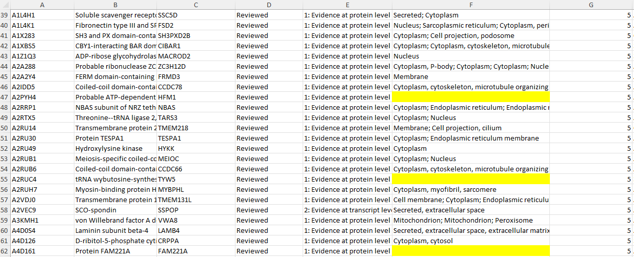
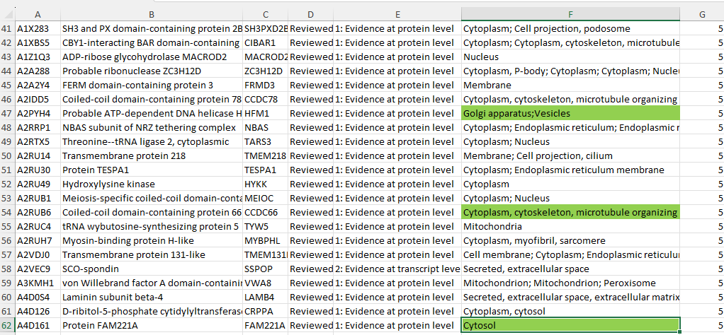
A snapshot of how the program used the second dataset(https://www.proteinatlas.org/about/download) to replace misssing values for 1827 proteins.
Link to the excel file after Data imputation : Cleaned_raw_1.xlsx
2. Removing Unnecessary Columns and Missing Values
The next step is to clean the data by removing unnecessary columns and any missing values. Since the Protein_Name and Gene_Name columns are redundant with UniProt_ID, I will remove them. I will also remove any rows containing missing values to ensure the dataset is complete.
import pandas as pd

file_path = r'dir_to_Cleaned_raw_1.xlsx'
df = pd.read_excel(file_path)

df = df.drop(columns=['Protein_Name', 'Gene_Name'])
df_cleaned = df.dropna()

output_path = r'path_to_save_cleaned_file.xlsx'
df_cleaned.to_excel(output_path, index=False)

print(f"Cleaned data (without 'Protein_Name' and 'Gene_Name') saved to {output_path}")
Link to the excel file after removing missing values and the two columns : Cleaned_raw_2.xlsx

Before

After
Note:Additional data cleaning could be performed; however, there is concern that removing certain features might negatively impact the models being developed. If further data cleaning is undertaken, updates will be applied accordingly
Visualization of the cleaned data
Here I will try to show few ways to visuzualize what I have in my protein data.
Data Viz-1
import pandas as pd
import matplotlib.pyplot as plt

file_path = r'path_to_cleaned_xlsx/csv_file'
df = pd.read_excel(file_path)

# Count unique values
value_counts = df['Protein_Existence'].value_counts()

plt.figure(figsize=(10, 6))
bars = value_counts.plot(kind='bar', color='lightseagreen')

plt.title('Protein Existence Distribution', fontsize=16)
plt.xlabel('Protein Existence Level', fontsize=14)
plt.ylabel('# of proteins', fontsize=14)

# Rotate x-axis labels
bars.set_xticklabels(bars.get_xticklabels(), rotation=45, ha='right')

max_value = value_counts.max()
plt.ylim(0, max_value + 0.1 * max_value)  # Add space above bars

# Hide top and right borders
bars.spines['top'].set_visible(False)
bars.spines['right'].set_visible(False)

# Add value labels on bars
for bar in bars.patches:
    bars.annotate(format(int(bar.get_height())), (bar.get_x() + bar.get_width() / 2, bar.get_height()),
                  ha='center', va='bottom', fontsize=12, color='black')

plt.tight_layout()
plt.show()
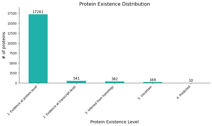
Figure 1: bar plot showing the distribution of protein existence levels, with counts for each evidence category. Most of the proteins have a evidence at a protein level.
Data Viz-2
import pandas as pd
import matplotlib.pyplot as plt
import seaborn as sns

file_path = r'path_to_cleaned_xlsx_or_csv_file'
df = pd.read_excel(file_path)

location_counts = df['Subcellular_Locations'].str.split(';|,').explode().str.strip().value_counts()

top_n = 15
top_locations = location_counts.nlargest(top_n)

plt.figure(figsize=(12, 8))
ax = sns.barplot(x=top_locations.values, y=top_locations.index, palette='viridis')

plt.title(f'Top {top_n} Subcellular Locations of Proteins', fontsize=16)
plt.xlabel('Protein Count', fontsize=12)
plt.ylabel('Subcellular Location', fontsize=12)

for i, v in enumerate(top_locations.values):
    plt.text(v, i, f' {v}', va='center')

# Remove top and right spines
ax.spines['top'].set_visible(False)
ax.spines['right'].set_visible(False)

plt.tight_layout()

output_path = r'C:\Users\micha\Downloads\upd\subcellular_locations_barplot.png'
plt.savefig(output_path, dpi=300, bbox_inches='tight')
print(f"Plot saved to {output_path}")

plt.show()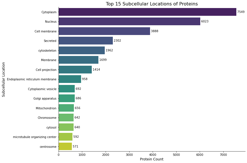
Figure 2: Shows top 15 locations the proteins localize in. From teh graph it is clear that the Cytoplasm is has a lot of proteins that aree found in it. Total number of unique subcellular locations ind the data is actually 268 and I have the link for subcellular_locations_frequency of all proteins.
Link to an excel file that shows subcellular_locations_frequency: subcellular_locations_frequency.xlsx
Data Viz-3
import pandas as pd
import matplotlib.pyplot as plt

file_path = r'path_to_cleaned_xlsx_or_csv_file'
df = pd.read_excel(file_path)

# Calculating the count of each sequence length
length_counts = df['Sequence_Length'].value_counts().sort_index()

#  scatter plot
plt.figure(figsize=(10, 6))
plt.scatter(length_counts.index, length_counts.values, color='orange', alpha=0.7)

# title and labels
plt.title('Scatter Plot of Protein Count vs Sequence Length', fontsize=16)
plt.xlabel('Sequence Length (Amino Acids)', fontsize=14)
plt.ylabel('Protein Count', fontsize=14)

# Removing parts of the graph
plt.gca().spines['top'].set_visible(False)
plt.gca().spines['right'].set_visible(False)

plt.tight_layout()
plt.show()
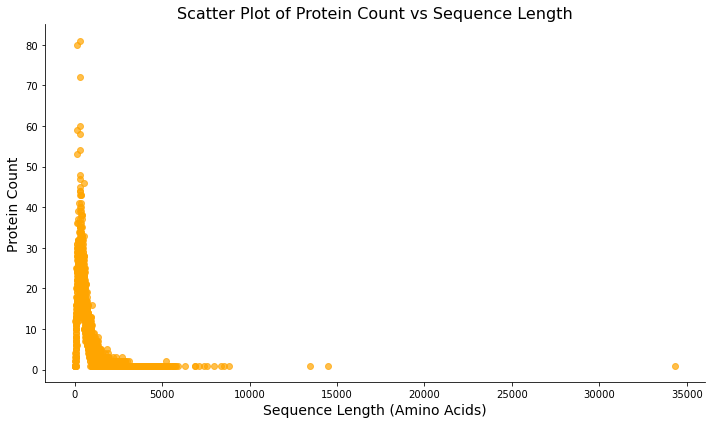
Figure 3: Scatterplot showing the distribution of protein lengths. This plot examines all human proteins in the database and displays the distribution of their lengths.
Data Viz-4
This will show the relative abundance of different amino acids across my protein dataset.
import pandas as pd
import seaborn as sns
import matplotlib.pyplot as plt

file_path = r'path_to_cleaned_xlsx_or_csv_file'
df = pd.read_excel(file_path)

# Column selection
aa_columns = ['Percent_A', 'Percent_C', 'Percent_D', 'Percent_E', 'Percent_F', 'Percent_G', 'Percent_H',
              'Percent_I', 'Percent_K', 'Percent_L', 'Percent_M', 'Percent_N', 'Percent_P', 'Percent_Q',
              'Percent_R', 'Percent_S', 'Percent_T', 'Percent_V', 'Percent_W', 'Percent_Y']

# Calculating the mean percentage for each amino acid
aa_means = df[aa_columns].mean().sort_values(ascending=False)

# Create a DataFrame with the mean percentages
aa_df = pd.DataFrame({'Amino Acid': aa_means.index.str.replace('Percent_', ''),
                      'Mean Percentage': aa_means.values})

# Creating the heatmap
plt.figure(figsize=(12, 8))
heatmap = sns.heatmap(aa_df.set_index('Amino Acid').T, annot=True, fmt='.2f', cmap='YlOrRd', cbar_kws={'label': 'Mean Percentage'})

plt.title('Heatmap of Mean Amino Acid Composition Across Proteins', fontsize=16)
plt.xlabel('Amino Acid', fontsize=12)
plt.ylabel('')  # Remove y-axis label as it's not needed
plt.tight_layout()

# Saving the figure
output_path = r'save_as_png '
plt.savefig(output_path, dpi=300, bbox_inches='tight')
print(f"Heatmap saved to {output_path}")

plt.show()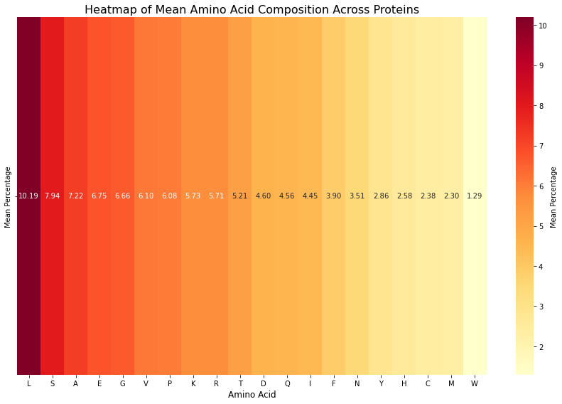
Figure 4: Heatmap of amino acid composition of the entire protein in the dataset. This heatmap represents 20 amino acids, with Leucine (L) showing the highest mean percentage and Tryptophan (W) showing the lowest mean percentage, consistent with findings in the literature.
Data Viz-5
import pandas as pd
import seaborn as sns
import matplotlib.pyplot as plt

file_path = r'path_to_cleaned_xlsx_or_csv_file'
df = pd.read_excel(file_path)

# Select proteins localized to the cell membrane
cell_membrane_proteins = df[df['Subcellular_Locations'].str.contains('Cell membrane', case=False, na=False)]

aa_columns = ['Percent_A', 'Percent_C', 'Percent_D', 'Percent_E', 'Percent_F', 'Percent_G', 'Percent_H',
              'Percent_I', 'Percent_K', 'Percent_L', 'Percent_M', 'Percent_N', 'Percent_P', 'Percent_Q',
              'Percent_R', 'Percent_S', 'Percent_T', 'Percent_V', 'Percent_W', 'Percent_Y']

# Calculate the mean percentage for each amino acid in cell membrane proteins
aa_means = cell_membrane_proteins[aa_columns].mean().sort_values(ascending=False)

# Create a DataFrame with the mean percentages
aa_df = pd.DataFrame({'Amino Acid': aa_means.index.str.replace('Percent_', ''),
                      'Mean Percentage': aa_means.values})

# Creates the heatmap
plt.figure(figsize=(12, 8))
heatmap = sns.heatmap(aa_df.set_index('Amino Acid').T, annot=True, fmt='.2f', cmap='Greens', cbar_kws={'label': 'Mean Percentage'})

plt.title('Heatmap of Mean Amino Acid Composition in Cell Membrane Proteins', fontsize=16)
plt.xlabel('Amino Acid', fontsize=12)
plt.ylabel('')
plt.tight_layout()

# Save the figure
output_path = r''
plt.savefig(output_path, dpi=300, bbox_inches='tight')
print(f"Heatmap saved to {output_path}")

# Prints the total number of cell membrane proteins
print(f"Number of cell membrane proteins: {len(cell_membrane_proteins)}")

plt.show()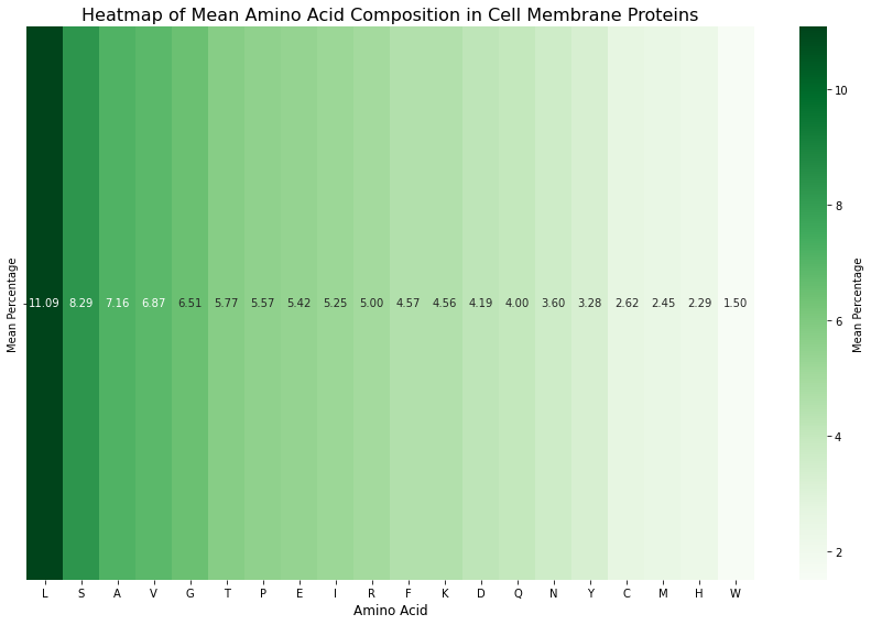
Figure 5: Heatmap of the amino acid composition of cell membrane proteins. This analysis focuses specifically on proteins located in the cell membrane. The data show that Valine (V) ranks higher in cell membrane proteins compared to Figure 4, which represents the amino acid composition of all proteins.
Data Viz-6
import pandas as pd
import seaborn as sns
import matplotlib.pyplot as plt

file_path = r'path_to_cleaned_xlsx_or_csv_file'
df = pd.read_excel(file_path)

# Select proteins localized to the nucleus
nuclear_proteins = df[df['Subcellular_Locations'].str.contains('Nucleus', case=False, na=False)]

aa_columns = ['Percent_A', 'Percent_C', 'Percent_D', 'Percent_E', 'Percent_F', 'Percent_G', 'Percent_H',
              'Percent_I', 'Percent_K', 'Percent_L', 'Percent_M', 'Percent_N', 'Percent_P', 'Percent_Q',
              'Percent_R', 'Percent_S', 'Percent_T', 'Percent_V', 'Percent_W', 'Percent_Y']

# Calculate the mean percentage for each amino acid in nuclear proteins
aa_means = nuclear_proteins[aa_columns].mean().sort_values(ascending=False)

# Create a DataFrame with the mean percentages
aa_df = pd.DataFrame({'Amino Acid': aa_means.index.str.replace('Percent_', ''),
                      'Mean Percentage': aa_means.values})

# Creates the heatmap
plt.figure(figsize=(12, 8))
heatmap = sns.heatmap(aa_df.set_index('Amino Acid').T, annot=True, fmt='.2f', cmap='Purples', cbar_kws={'label': 'Mean Percentage'})

plt.title('Heatmap of Mean Amino Acid Composition in Nuclear Proteins', fontsize=16)
plt.xlabel('Amino Acid', fontsize=12)
plt.ylabel('')  # Remove y-axis label as it's not needed
plt.tight_layout()

# Save the figure
output_path = r''
plt.savefig(output_path, dpi=300, bbox_inches='tight')
print(f"Heatmap saved to {output_path}")

# Prints the total number of cell membrane proteins
print(f"Number of nuclear proteins: {len(nuclear_proteins)}")

plt.show()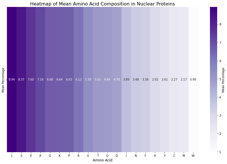
Figure 6: Heatmap of the amino acid composition of nuclear proteins. Lysine (K) appears at a higher level compared to Figure 4, which shows the amino acid composition of all proteins.
Data Viz-7
import pandas as pd
import matplotlib.pyplot as plt
import seaborn as sns


file_path = r'path_to_cleaned_xlsx_or_csv_file'
df = pd.read_excel(file_path)

#scatter plot
plt.figure(figsize=(12, 8))
ax = sns.scatterplot(x='Sequence_Length', y='Molecular_Weight', data=df, alpha=0.6)

#trend line
sns.regplot(x='Sequence_Length', y='Molecular_Weight', data=df, scatter=False, color='red')

# Customizing the plot
plt.title('Correlation Between Protein Length and Molecular Weight', fontsize=16)
plt.xlabel('Sequence Length (Number of Amino Acids)', fontsize=12)
plt.ylabel('Molecular Weight (Da)', fontsize=12)

ax.spines['top'].set_visible(False)
ax.spines['right'].set_visible(False)

# correlation coefficient with three significant figures
correlation = df['Sequence_Length'].corr(df['Molecular_Weight'])
correlation_formatted = f'{correlation:.3g}'
plt.text(0.05, 0.95, f'Correlation: {correlation_formatted}', transform=plt.gca().transAxes,
         fontsize=12, verticalalignment='top')

plt.tight_layout()
plt.show()
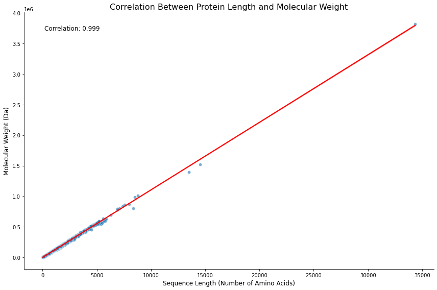
Figure 7: Scatter Plot with Regression Line: This scatter plot shows the relationship between amino acid sequence length and molecular weight (in Daltons/Da). The regression line indicates that as the sequence length increases, the molecular weight also increases. This simple analysis confirms that the data follows the expected trend.
Data Viz-8
import pandas as pd
import matplotlib.pyplot as plt
import seaborn as sns

file_path = r'path_to_cleaned_xlsx_or_csv_file'
df = pd.read_excel(file_path)

# Locations to compare
locations = ['Cytoplasm', 'Nucleus', 'Lysosome', 'Mitochondrion', 'Secreted', 'Endoplasmic reticulum', 'Golgi apparatusDataframe with isoelectric points for each location
isoelectric_data = []
for loc in locations:
    loc_proteins = df[df['Subcellular_Locations'].str.contains(loc, case=False, na=False)]
    isoelectric_data.extend([(loc, pi) for pi in loc_proteins['Isoelectric_Point']])

isoelectric_df = pd.DataFrame(isoelectric_data, columns=['Location', 'Isoelectric_Point'])

#box plot
plt.figure(figsize=(12, 6))
sns.boxplot(x='Location', y='Isoelectric_Point', data=isoelectric_df)

# plot
plt.title('Isoelectric Points by Subcellular Location', fontsize=16)
plt.xlabel('Subcellular Location', fontsize=12)
plt.ylabel('Isoelectric Point', fontsize=12)
plt.xticks(rotation=45, ha='right')
plt.tight_layout()

#
output_path = r''
plt.savefig(output_path, dpi=300, bbox_inches='tight')
plt.show()
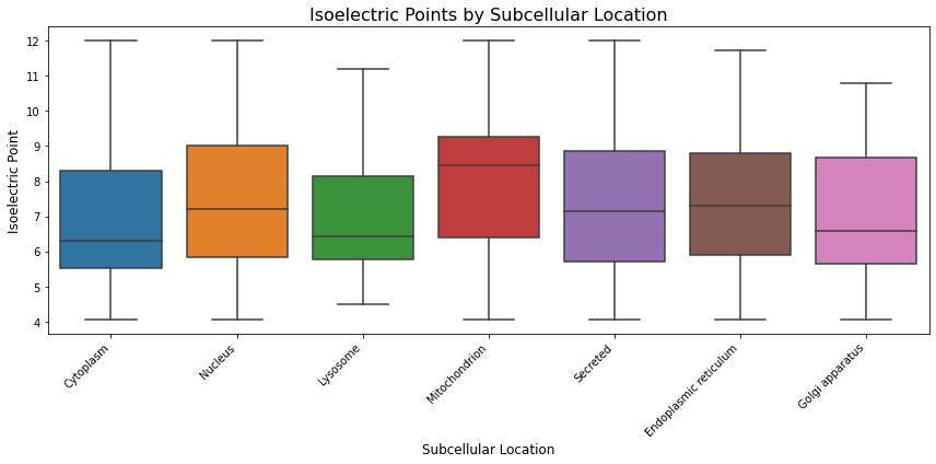
Figure 7: Box Plot of Isoelectric Points for Proteins Across Different Subcellular Locations. The box plot shows that proteins in the lysosome tend to have lower (more acidic) isoelectric points compared to those in the mitochondrion. This suggests that lysosomal proteins are generally more acidic than mitochondrial proteins.
Data Viz-9
import pandas as pd
import matplotlib.pyplot as plt
import seaborn as sns
import numpy as np

file_path = r'path_to_cleaned_xlsx_or_csv_file'
df = pd.read_excel(file_path)

# List of amino acids
amino_acids = 'ACDEFGHIKLMNPQRSTVWY'

# Select columns with amino acid percentages
aa_columns = [f'Percent_{aa}' for aa in amino_acids]

# Calculating correlation matrix
correlation_matrix = df[aa_columns].corr()

# Create a mask for the upper triangle
mask = np.triu(np.ones_like(correlation_matrix, dtype=bool))

# matplotlib figure
plt.figure(figsize=(12, 10))

# Create heatmap
sns.heatmap(correlation_matrix, mask=mask, cmap='coolwarm', vmin=-1, vmax=1, center=0,
            square=True, linewidths=.5, cbar_kws={"shrink": .5}, annot=True, fmt='.2f')

# Customizing the plot
plt.title('Correlation of Amino Acid Percentages in Proteins', fontsize=16)
plt.tight_layout()

# Saving the figure
output_path = r'C:\Users\micha\Downloads\upd\amino_acid_correlation_heatmap.png'
plt.savefig(output_path, dpi=300, bbox_inches='tight')
print(f"Heatmap saved to {output_path}")

plt.show()
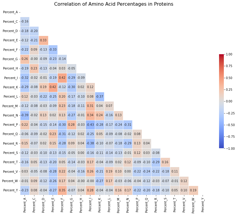
Figure 8: Correlation Heatmap of Amino Acid Percentages in Proteins: This heatmap shows how often two amino acids are found together in proteins. A value close to 1 means that if one amino acid is present in high amounts, the other is likely to be present too. A value close to -1 means that if one amino acid is present in high amounts, the other is likely to be low. Values around 0 suggest there is no clear pattern between the two amino acids.
import pandas as pd
import matplotlib.pyplot as plt
import seaborn as sns

file_path = r'path_to_cleaned_xlsx_or_csv_file'
df = pd.read_excel(file_path)

plt.figure(figsize=(12, 6))
hist = sns.histplot(data=df, x='Annotation_Score', bins=30, kde=False, color=sns.color_palette("Reds", as_cmap=True)(0.7))

for patch in hist.patches:
    height = patch.get_height()
    if height > 0:
        hist.text(patch.get_x() + patch.get_width() / 2, height + 0.5, int(height), ha="center", va="bottom", fontsize=10)

hist.spines['top'].set_visible(False)
hist.spines['right'].set_visible(False)
hist.spines['left'].set_visible(False)
hist.spines['bottom'].set_position('zero')

plt.xlabel('Annotation Score', fontsize=12)
plt.ylabel('Count', fontsize=12)

plt.tight_layout()
plt.show()
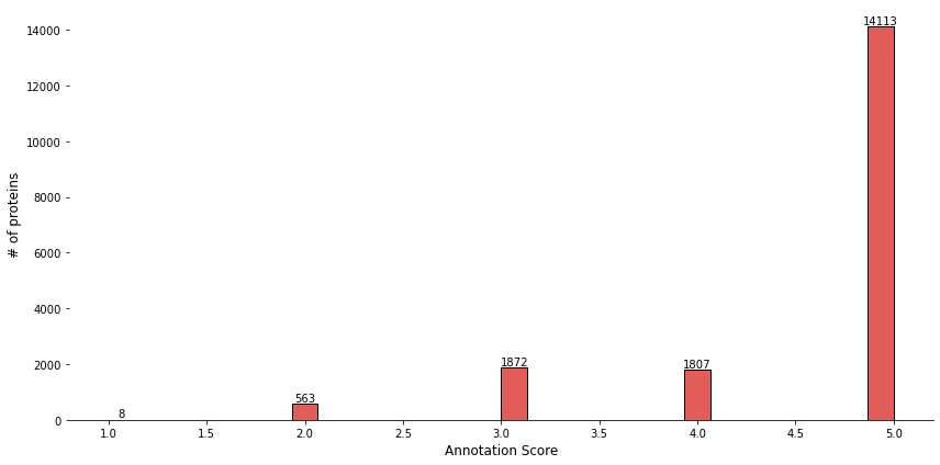
Figure 9: Distribution of Annotation Scores: The histogram highlights the overwhelming majority of proteins (14,113) receiving an annotation score of 5.0. This suggests that most proteins in the dataset are highly annotated, with significantly fewer proteins receiving lower annotation scores.
import pandas as pd
import matplotlib.pyplot as plt
import seaborn as sns
import numpy as np

file_path = r'path_to_cleaned_xlsx_or_csv_file'
df = pd.read_excel(file_path)

amino_acids = 'ACDEFGHIKLMNPQRSTVWY'
max_length = 50

def count_amino_acids(sequence, max_length):
    counts = np.zeros((len(amino_acids), max_length))
    for i, aa in enumerate(sequence[:max_length]):
        if aa in amino_acids:
            counts[amino_acids.index(aa), i] += 1
    return counts

total_counts = np.zeros((len(amino_acids), max_length))

for sequence in df['Amino_Acid_Sequence']:
    if isinstance(sequence, str):
        total_counts += count_amino_acids(sequence, max_length)

percentages = total_counts / total_counts.sum(axis=0) * 100

plt.figure(figsize=(20, 10))
sns.heatmap(percentages, xticklabels=range(1, max_length+1), yticklabels=list(amino_acids),
            cmap='YlOrRd', cbar_kws={'label': 'Percentage'})
plt.title('Amino Acid Frequency by Position', fontsize=16)
plt.xlabel('Position in Sequence', fontsize=12)
plt.ylabel('Amino Acid', fontsize=12)

plt.show()
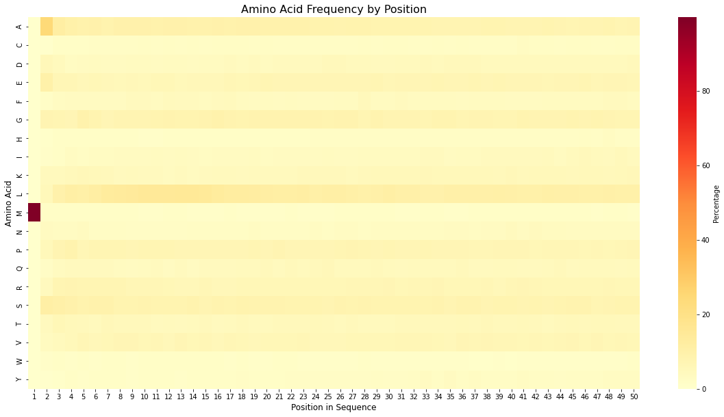
Figure 10: This heatmap shows the relative frequency (percentage) of each amino acid (y-axis) at each position (x-axis) within the first 50 amino acids of the sequences in the dataset. For visualization purposes, a window of the first 50 amino acids was selected, but the result remains consistent when the window is expanded. Methionine (M) is the first amino acid in nearly all proteins, appearing almost 100% of the time(the one in the dark brown color on the left side of the image at position #1).
Summary
This is just the beginnig. Mork work will be done to improve this to that the model has the beast avaialble data to make predictions on where any given protein is likley to be localized.
