This is a data mining technique that is used to discover interesting relationships or patterns in large datasets. Specifically, it aims to find associations between different items or events that frequently occur together.There are three most fundamental metrics: 1) Support 2) Confidence 3) Lift
Breif explanation of these three key metrics guiding ARM:
Lift: Lift helps determine whether the association is stronger than random chance. For example, a lift greater than 1 indicates that the presence of a particular amino acid pattern increases the likelihood of a protein being in a specific localization. For example, if a lift of 1.5 is calculated, it means that the proteins with those amino acids are 1.5 times more likely to localize to that specific part of the cell than by chance.
Support: This measures how frequently a particular combination of items (in this case, amino acids or localization patterns) appears in the dataset. For example, if certain amino acids are found in 30% of proteins that localize to the nucleus, the support for this itemset is 0.30. This tells us how common that association is within the dataset.
Confidence: Confidence measures the reliability of an association. It answers the question: given that a protein contains certain amino acids (A), how likely is it to be found in a specific subcellular location (B)? For instance, if 70% of proteins with a certain amino acid profile are localized to the cytoplasm, the confidence for that rule is 0.70.

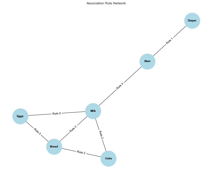
Figure 1: A network graph shows the relationships between items based on the discovered association rules, with nodes representing items and edges representing rules connecting them. The labels on the edges indicate which rule each connection represents, depicting how different items are associated in the dataset.Due to its multiple connections in the Association Rule Network, it tells us that milk is a central item in the dataset, frequently purchased alongside various other products like Eggs, Bread, and Coke.

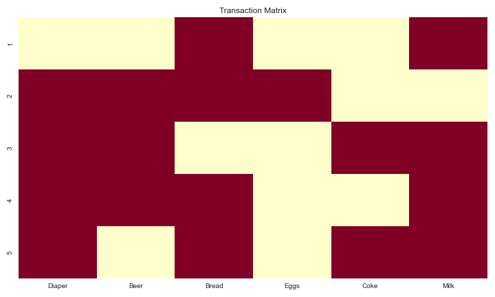
Figure 2 : A heatmap that visualizes the presence (dark red) or absence (light yellow) of items in each transaction, with rows representing transactions and columns representing items. It provides a quick overview of which items frequently appear together across different transactions.
Data Prep
import pandas as pd

# Loading the data without labels
file_path = r'path_to_amino_acid_seq_Nucleus_Cytoplasm_Cell_membrane_LABELS_REMOVED.xlsx'
data = pd.read_excel(file_path)

# Converting the percentages to decimal format
data = data / 100

# Setting the binarization threshold
threshold = 0.1

# Applying binarization: convert values above threshold to 1 and below to 0
binary_data = data.applymap(lambda x: 1 if x > threshold else 0)

# Saving the binarized data to a new Excel file
binary_file_path = r'path_to_binary_amino_acid_data.xlsx'
binary_data.to_excel(binary_file_path, index=False)

# Showing a tiny bit of the the binarized data
print(binary_data.head())
Binarized excel file link: binary_amino_acid_data.xlsx

Screenshot of the binarized data from above
I binarized the amino acid composition data to create a transaction-like format. Each protein is treated as a transaction, and each amino acid is treated as an item. This format is required for the Apriori algorithm to identify frequent amino acid patterns across proteins and generate useful association rules.
The transaction data consists of amino acid compositions (represented as binary values) for proteins localized to different subcellular regions (e.g., nucleus, cytoplasm, cell membrane). Each protein would be treated as a “transaction,” and each amino acid type (e.g., A, C, D, E) would be treated as a “product” or “item” in the transaction.
Apriori Algorithm
# Loading libraries needed
library(arules)
library(arulesViz)
library(readxl)
library(htmlwidgets)

# Setting my working directory
setwd("path")

# Load your binary data from the Excel file
file_path <- "path_to_binary_amino_acid_data.xlsx"
data <- read_excel(file_path, sheet = 1)

# Converting the data to a transaction format
binary_data <- as(as.matrix(data), "transactions")

# Explore the loaded data
# just to see
summary(binary_data)

#1: Run the Apriori algorithm with adjusted support and confidence thresholds
# Adjust the support and confidence to ensure 15+ rules
rules <- apriori(binary_data, parameter = list(support = 0.004, confidence = 0.4, minlen = 2))

# Checking how many rules were generated
cat("Number of rules generated:", length(rules), "\n")

#2: Sorting rules by lift, confidence, and support
# Sorting and printing top 15 rules by Lift
sorted_rules_by_lift <- sort(rules, by = "lift", decreasing = TRUE)
cat("\nTop 15 rules sorted by Lift:\n")
inspect(head(sorted_rules_by_lift, 15))

# Sorting and printing top 15 rules by Confidence
sorted_rules_by_confidence <- sort(rules, by = "confidence", decreasing = TRUE)
cat("\nTop 15 rules sorted by Confidence:\n")
inspect(head(sorted_rules_by_confidence, 15))

# Sorting and printing top 15 rules by Support
sorted_rules_by_support <- sort(rules, by = "support", decreasing = TRUE)
cat("\nTop 15 rules sorted by Support:\n")
inspect(head(sorted_rules_by_support, 15))

#3: Visualizing the top 15 rules by lift
if (length(sorted_rules_by_lift) > 0) {
    top_rules <- head(sorted_rules_by_lift, 15)
    plot_obj <- plot(top_rules, method = "graph", engine = "htmlwidget")

    # Saving the plot as an interactive HTML file
    htmlwidgets::saveWidget(plot_obj, file = "top_15_rules.html")
    cat("Interactive_plot_or_chart saved as 'top_15_rules.html'.\n")
} else {
    cat("No rules available for plotting.\n")
}

# Step 4: Printing most frequent items in the rules
cat("\nTop 10 most frequent items in rules:\n")
itemFrequencyPlot(binary_data, topN = 10, type = "absolute")

# Step 5: Printing summary of the binary transaction data
cat("\nSummary of Binary Transaction Data:\n")
summary(binary_data)
Refrence: Dr. Ami Gates, CU Boulder(https://gatesboltonanalytics.com/?page_id=268)
Top 15 Association Rules for Amino Acid Percentages(it is interactive)
This graph visualizes the top 15 association rules identified in the amino acid percentage data, based on the Apriori algorithm. The rules were generated using a support threshold of 0.004 (0.4%), a confidence threshold of 0.4 (40%), and a minimum rule length of 2. The nodes represent individual amino acid percentages, while the arrows illustrate the direction and strength of the association, with the thickness of the lines indicating the strength (lift) of the rule. These rules help uncover relationships between amino acids in different proteins, providing insight into common patterns.
Ineterpreting the chart above
When hovering over Rule 1 in the association graph, we can see the following insights:
- Support: 0.00687 – This indicates that 0.687% of all transactions (protein compositions) contain both
Percent_P,Percent_R, andPercent_A. - Confidence: 0.653 – This means that 65.3% of the time, if
Percent_PandPercent_Rare present,Percent_Awill also be present. - Lift: 5 – The lift value suggests that the presence of
Percent_PandPercent_Rmakes it 5 times more likely thatPercent_Awill also occur compared to if they were independent. - Count: 32 – This is the actual number of transactions (rows in the data) that support this rule.
Note(just a reminder): The values like Percent_A, Percent_P, and Percent_R represent the percentage of each specific amino acid(1 of 20) in a given protein.
Association Rule Localization Analysis for Predicting Subcellular Protein Locations
Note: I thought of adding this(even though, I don’t think is required) as it can be used as an addition to the analysis of association rules. By mapping the rules to specific subcellular localizations (Nucleus, Cytoplasm, and Cell Membrane), this script helps identify which amino acid patterns are most predictive of a particular protein’s location within the cell.
import pandas as pd

# Loading the labeled data containing amino acid compositions with subcellular locations
file_path = 'path_to_amino_acid_seq_Nucleus_Cytoplasm_Cell_membrane_WITH_LABELS.xlsx'
labeled_data = pd.read_excel(file_path)

# Loading the rules output from the previous association rule analysis
rules_output = pd.read_excel('path_to_rules_output.xlsx')

# Defining a function to check if a rule's lhs (left-hand side) and rhs (right-hand side) amino acids are matching the protein composition
def rule_matches_protein(rule, protein_data):
    # Splitting the rule into lhs and rhs components
    lhs_rhs = rule.strip('{}').split('=>')
    lhs = lhs_rhs[0].replace('{', '').replace('}', '').split(',')
    rhs = lhs_rhs[1].strip().replace('{', '').replace('}', '')

    # Removing any extra spaces in lhs and rhs
    lhs = [item.strip() for item in lhs]
    rhs = rhs.strip()

    try:
        # Ensuring 'Percent_' prefix for columns to match the data format
        lhs_columns = [aa if aa.startswith('Percent_') else f'Percent_{aa}' for aa in lhs]
        rhs_column = rhs if rhs.startswith('Percent_') else f'Percent_{rhs}'

        # Checking if all amino acids in the lhs have non-zero percentages
        lhs_matches = all(protein_data[aa] > 0 for aa in lhs_columns)

        # Checking if the rhs amino acid has a non-zero percentage
        rhs_matches = protein_data[rhs_column] > 0
    except KeyError:
        return False

    return lhs_matches and rhs_matches

# Initializing a dictionary to store counts for each subcellular location
localization_counts = {'Nucleus': [], 'Cytoplasm': [], 'Cell membrane': []}

# Iterating over each rule and counting occurrences in proteins from different localizations
for rule in rules_output['rules']:
    for loc in ['Nucleus', 'Cytoplasm', 'Cell membrane']:
        # Filtering proteins by subcellular location
        localized_proteins = labeled_data[labeled_data['Subcellular_Location'] == loc]

        # Counting how many proteins match the rule
        match_count = sum(localized_proteins.apply(lambda row: rule_matches_protein(rule, row), axis=1))
        localization_counts[loc].append(match_count)

# Creating a DataFrame to store the localization counts for each rule
localization_df = pd.DataFrame(localization_counts, index=rules_output['rules'])

# Adding a column to identify the dominant location for each rule based on the highest match count
localization_df['Dominant_Location'] = localization_df.idxmax(axis=1)

# Saving the results to an Excel file
output_file = 'path_to_rule_dominant_location_analysis.xlsx'
localization_df.to_excel(output_file)
print(f'Dominant location analysis saved to {output_file}')
Link to the excel file created :rule_dominant_location_analysis.xlsx

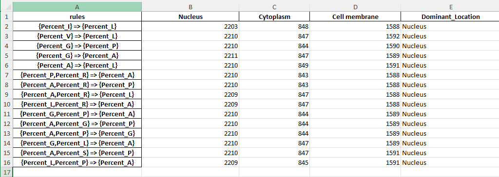
Screenshot of the excel file created
This Python script above identifies which subcellular location (nucleus, cytoplasm, or cell membrane) is most strongly associated with each of the top association rules derived from the amino acid composition data. It does so by comparing how often each rule matches proteins in different subcellular locations, providing insight into which rules best predict the localization of proteins based on their amino acid content.
Conclusions
The analysis of amino acid percentages using association rule mining revealed several patterns that predominantly predict nuclear localization. All of the top 15 rules had a strong association with proteins localized in the nucleus, as seen by the dominant “Nucleus” prediction across all rules. The confidence and lift values indicate that specific combinations of amino acids, such as {Percent_P, Percent_R} => {Percent_A}, are strongly indicative of nuclear proteins. No significant patterns emerged for cytoplasmic or cell membrane localization, suggesting that the data, in its current form, is more predictive of nuclear proteins. Further refinement of the rules or exploration of additional features may be necessary to uncover patterns linked to cytoplasm or cell membrane proteins.
