PCA or Principal Component Analysis is a method for reducing the number of variables in a dataset by transforming them into a smaller set of new variables, called principal components. To me, it is like asking, “How can I simplify this data by getting rid of less important stuff while keeping most of the original variability?”. If we break down the acronym PCA, the ‘PC’ stands for ‘principal component,’ which refers to a new variable that highlights the most significant patterns in the original data. By focusing on these principal components, PCA allows us to work with simplified versions of complex datasets without losing essential information needed for effective analysis and decision making. So, PCA is a very important process of data analysis because it makes data much cleaner, less computationally intensive, and easier to interpret and visualize, while still preserving the most critical information. This ability to reduce dimensionality while retaining most of the variance is what makes it so useful.
Example using the Iris dataset
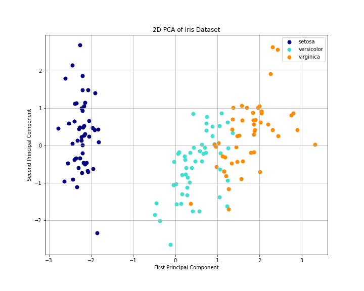
Figure 1: This 2D PCA plot visualizes the Iris dataset, projecting it onto the first two principal components. The three Iris species (setosa, versicolor, and virginica) are clearly distinguishable, with setosa forming a tight, well-separated cluster, while versicolor and virginica show some overlap but are still largely distinct, demonstrating PCA’s effectiveness in reducing dimensionality while preserving important differences between classes.
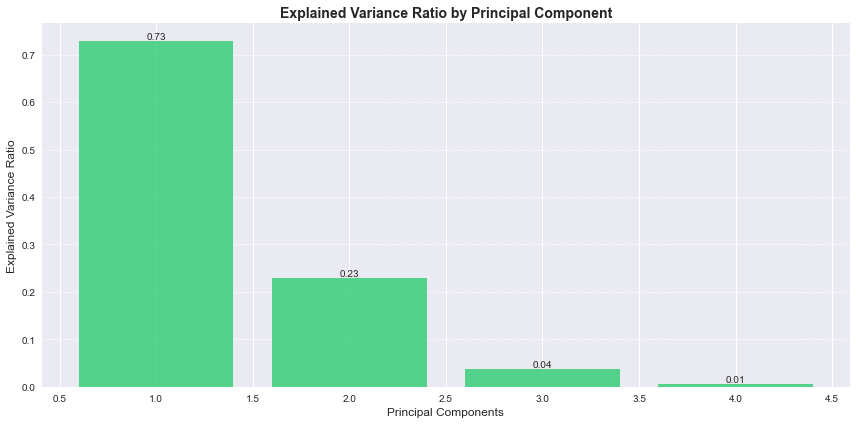
Figure 2: This bar graph shows the explained variance ratio for each principal component in the Iris dataset. The first two components together account for 96% of the total variance, with the first component alone explaining 73%, demonstrating that most of the dataset’s important information can be captured in just two dimensions.
Now to my data
Python Script for Extracting Amino Acid Composition Data for Principal Component Analysis (PCA) Preparation
-This code extracts specific quantitiative data(Acid Composition Data) from the original cleaned data.
import pandas as pd
# Loading data
file_path = r'path_to_Cleaned_raw_2.csv'
data = pd.read_csv(file_path)
# Amino acid columns to be extracted from the original file "Cleaned_raw_2.csv"
amino_acid_columns = ['Percent_A', 'Percent_C', 'Percent_D', 'Percent_E', 'Percent_F',
                      'Percent_G', 'Percent_H', 'Percent_I', 'Percent_K', 'Percent_L',
                      'Percent_M', 'Percent_N', 'Percent_P', 'Percent_Q', 'Percent_R',
                      'Percent_S', 'Percent_T', 'Percent_V', 'Percent_W', 'Percent_Y']
# Extracts the relevant data
amino_acid_data = data[amino_acid_columns]

# Save the extracted data
output_file_path = r'path_to_extracted_amino_acid_data.csv'
amino_acid_data.to_csv(output_file_path, index=False)
print('Extraction complete.')

Figure 3: Screenshot of the dataset used for PCA analysis. This figure displays the percentage composition of all 20 amino acids for each protein in the dataset. The data includes columns labeled from Percent_A to Percent_Y, representing the amino acid percentages. This quantitative data was extracted from the full dataset ( Cleaned_raw_2.csv) and will serve as the input for the PCA analysis.
Link to the data that will be used for PCA: extracted_protein_aa_data.xlsx
Principal Component Analysis (PCA) for Dimensionality Reduction and Visualization of Amino Acid Composition
-Used Sklearn StandardScaler to normalize the data
import pandas as pd
from sklearn.preprocessing import StandardScaler
from sklearn.decomposition import PCA
import matplotlib.pyplot as plt
from mpl_toolkits.mplot3d import Axes3D

# Loading data
file_path = r'path_to_extracted_amino_acid_data.csv'
data = pd.read_csv(file_path)

# Part 1: Standardizing using StandardScaler
scaler = StandardScaler()
X_scaled = scaler.fit_transform(data)

# Part 2: Performing PCA with n_components=2
pca_2d = PCA(n_components=2)
X_pca_2d = pca_2d.fit_transform(X_scaled)

# Part 3: Performing PCA with n_components=3
pca_3d = PCA(n_components=3)
X_pca_3d = pca_3d.fit_transform(X_scaled)

# Part 4: Enhanced Plot for 2D PCA Results
plt.figure(figsize=(10,7))
plt.scatter(X_pca_2d[:, 0], X_pca_2d[:, 1], c=X_pca_2d[:, 0], cmap='viridis', s=50, alpha=0.7, edgecolors='k')
plt.colorbar(label='Principal Component 1 Value')
plt.xlabel('Principal Component 1', fontsize=12)
plt.ylabel('Principal Component 2', fontsize=12)
plt.title('2D PCA of Amino Acid Percentages', fontsize=15)
plt.grid(True, linestyle='--', alpha=0.7)
plt.tight_layout()
plt.show()

# Part 5: Enhanced Plot for 3D PCA Results
fig = plt.figure(figsize=(12,8))
ax = fig.add_subplot(111, projection='3d')
scatter = ax.scatter(X_pca_3d[:, 0], X_pca_3d[:, 1], X_pca_3d[:, 2], c=X_pca_3d[:, 0], cmap='plasma', s=60, alpha=0.8, edgecolors='k')

# Adding labels
ax.set_xlabel('Principal Component 1', fontsize=12)
ax.set_ylabel('Principal Component 2', fontsize=12)
ax.set_zlabel('Principal Component 3', fontsize=12)
ax.set_title('3D PCA of Amino Acid Percentages', fontsize=15)

# Add colorbar
cbar = fig.colorbar(scatter, ax=ax, shrink=0.5, aspect=5)
cbar.set_label('Principal Component 1 Value')

plt.tight_layout()
plt.show()

# Part 6: Printing the explained variance ratios for 2D and 3D PCA
explained_variance_2d = pca_2d.explained_variance_ratio_
explained_variance_3d = pca_3d.explained_variance_ratio_

print(f'Explained variance for 2D PCA: {explained_variance_2d}')
print(f'Explained variance for 3D PCA: {explained_variance_3d}')

# Part 7: Showing cumulative explained variance for more dimensions
pca_full = PCA().fit(X_scaled)
cumulative_variance = pca_full.explained_variance_ratio_.cumsum()
print(f'Cumulative variance explained by all components: {cumulative_variance}')

# Finding the number of components required to retain 95% of the variance
n_components_95 = next(i for i, total in enumerate(cumulative_variance) if total >= 0.95) + 1
print(f'Number of components needed to retain at least 95% of the variance: {n_components_95}')

# Part 8: Printing the top 3 eigenvalues
eigenvalues = pca_full.explained_variance_[:3]
print(f'Top 3 eigenvalues (explained variance): {eigenvalues}')
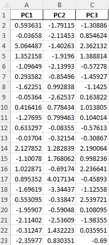
Screenshot of the data after PCA
PCA Results Summary

Screenshot of the Python code output, which is also provided below
Explained variance for 2D PCA: [0.16636706, 0.13373548]
Explained variance for 3D PCA: [0.16636688, 0.13373489, 0.08389696]
Cumulative variance explained by all components:
[0.16636708, 0.30010318, 0.38401062, 0.45376562, 0.51578499, 0.5661034, 0.61436155, 0.65841657, 0.69731595, 0.73468425, 0.7703088, 0.80404245, 0.83703194, 0.86961409, 0.90090695, 0.93065588, 0.95560999, 0.97910762, 1. 1. ]
Number of components needed to retain at least 95% of the variance: 17
Top 3 eigenvalues (explained variance): [3.32752271, 2.67486771, 1.67824032]
2D and 3D Visualization
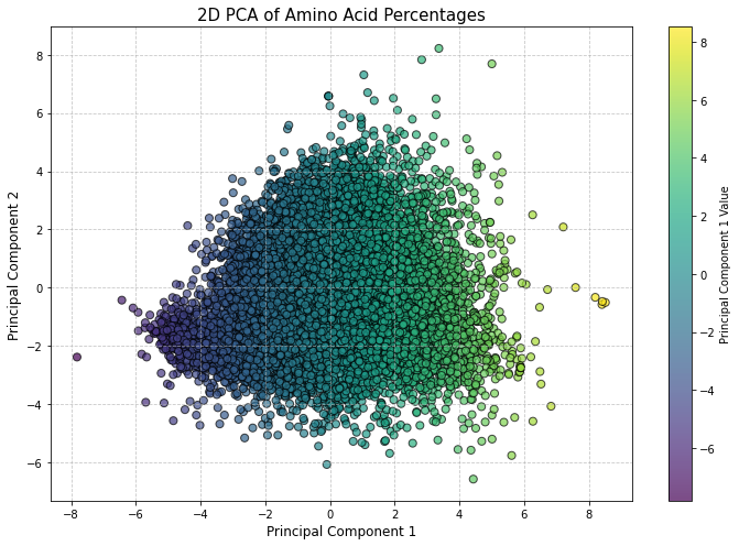
Figure 4: This 2D PCA plot shows the distribution of proteins based on their amino acid composition, with Principal Component 1 explaining 16.63% and Principal Component 2 explaining 13.37% of the total variance. Each point represents a protein, with the color gradient indicating values along the first principal component. This plot captures around 30% of the total variance.
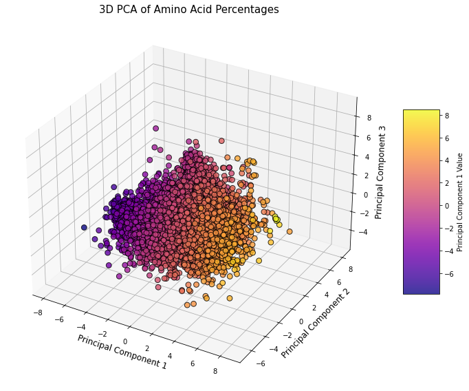
Figure 5: This 3D PCA plot shows the distribution of proteins based on their amino acid composition, with Principal Component 1 explaining 16.63%, Principal Component 2 explaining 13.37%, and Principal Component 3 explaining 8.39% of the total variance. Each point represents a protein, and the color gradient reflects values along the first principal component. This 3D plot captures approximately 38.4% of the total variance.
Summary
The 2D PCA retains about 30% of the total variance, while the 3D PCA captures 38.4% of the variance in the amino acid composition of the proteins. To retain at least 95% of the variance, we need 17 components, which indicates to me that the data is highly multidimensional. The top three eigenvalues, which represent the variance explained by the most important components, are 3.33, 2.67, and 1.68.
